Spatial Aggregation

When dealing with spatial data in sales and / or social science context it is common that data are reported per administrative units (defined as polygons).

This has its benefits – administrative units, such as counties, states or districts, are generally well understood by our users, and make a good base for convincing choropleth maps – but also disadvantages. Administrative areas differ greatly in size and population and are not always good inputs for modelling.

To remedy this I propose three different approaches for spatial aggregation of data reported per administrative area polygons:

based on spatial buffers
based on Voronoi polygons
based on equal distance grid cells

As my post is about general techniques, and not a specific implementation, any spatial data object would do. I am choosing to demonstrate the techniques on the North Carolina shapefile that ships with {sf} package, based on nothing else than its general availability (nc.shp is the Iris of spatial data).

All the techniques are distance related a projected CRS is thus required. Being an European, metric born & raised, am choosing one based on US Survey Feet; I confess I am mildly amused by the rationale behind 660 feet to a furlong.

My first step is creating of 3 spatial objects:

county data of births in the years 1979 to 1984 from the nc.shp dataset; note that I calculate a column of county area (in squared survey feet); this will come handy later on
NC state boundaries, obtained by dissolving the nc.shp polygons
point data of three semi-random cities in NC; these will be basis for the aggregation

library(sf)
library(dplyr)
library(ggplot2)

# NC counties - a shapefile shipped with the sf package
counties <- st_read(system.file("shape/nc.shp", package = "sf"), quiet = T) %>% 
  select(BIR79)  %>% # a single variable: births for period 1979-84
  st_transform(crs = 6543) %>%  # a quaint local projection
  mutate(cty_area = units::drop_units(st_area(.))) # county area (in feet)
  
# NC state borders
state <- counties %>% 
  summarize()

# three semi-random cities in NC
points <- data.frame(name = c("Raleigh", "Greensboro", "Wilmington"),
                     x = c(-78.633333, -79.819444, -77.912222),
                     y = c(35.766667, 36.08, 34.223333)) %>% 
  st_as_sf(coords = c("x", "y"), crs = 4326) %>% 
  st_transform(crs = st_crs(counties))  # same as counties

As I will be drawing a chart of NC births a lot I am creating a convenience function to simplify this task (and to not repeat myself).

The first step is to apply this function to the raw county data, and in doing so gain an overall understanding of the births metric.

# define the function
chart <- function(dataframe) {
  ggplot() +
  geom_sf(data = dataframe, aes(fill = BIR79), alpha = .5, lwd = .25) +
  geom_sf(data = state, lwd = .75, fill = NA) + 
  geom_sf(data = points, color = "red", size = 2) +
  scale_fill_gradient(trans = "log10", 
                      low = "white",
                      high = "firebrick",
                      labels = scales::comma_format()) +
  labs(fill = "Births\n1979 - 84") +
  guides(fill = guide_legend(override.aes = list(alpha = 0.5))) +
  theme(legend.text.align = 1,
        legend.title.align = 1/2)
}

# apply it to raw county data
chart(counties)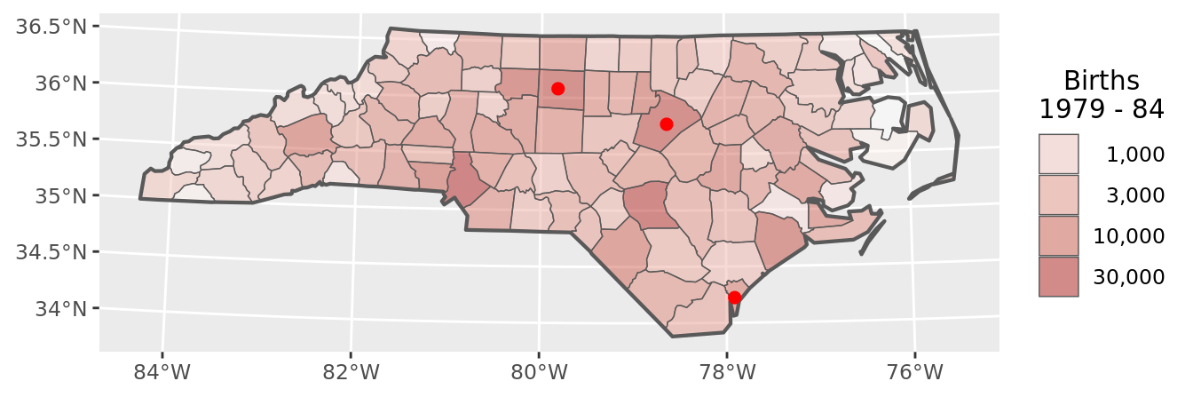

The second step is to prepare spatial objects that will be basis of our future aggregation.

Buffers are the easiest, produced by a call to sf::st_buffer() on our points data, with second argument of distance — in our case 50 miles – and then cut to shape via sf::st_intersection() with the shape of NC state.

# create the buffers object
buffers <- st_buffer(points, 50 * 5280) %>% # 50 miles circle
  st_intersection(state) # cut to shape of NC state

# display the buffers
ggplot() +
  geom_sf(data = buffers, aes(fill = name), alpha = .5) +
  geom_sf(data = state, lwd = .75, fill = NA) + 
  geom_sf(data = points, color = "red", pch = 4, size = 2) +
  labs(fill = "Zone")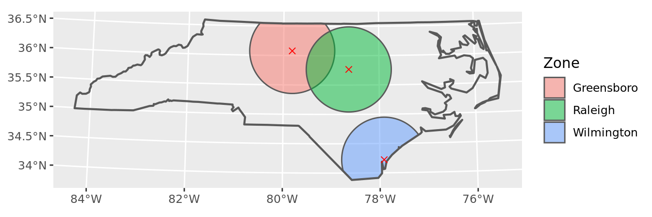

The Voronoi polygons are somewhat more challenging, as the geometry creation necessitates more steps; the sf::st_voronoi() function requires as argument a sfc object of MULTIPOINT type. This means first extracting geometry, i.e. without any data, from the sf object of points, and then merging of the list of multiple points to a single multipoint object via sf::st_union().

The resulting polygon is then cut to shape of NC state, converted back to sf class and joined with the original point data to re-gain the dimension of city names it lost in previous steps.

# create the voronoi object
voronoi <- points %>% 
  st_geometry() %>% # to get sfc from sf
  st_union() %>% # to get a sfc of MULTIPOINT type
  st_voronoi(envelope = st_geometry(state)) %>% # NC sized Voronoi polygon
  st_collection_extract(type = "POLYGON") %>% # a list of polygons
  st_sf() %>% # from list to sf object
  st_intersection(state) %>% # cut to shape of NC state
  st_join(points) # put names back

# display the Voronoi polygons
ggplot() +
  geom_sf(data = voronoi, aes(fill = name), alpha = .5) +
  geom_sf(data = state, lwd = .75, fill = NA) + 
  geom_sf(data = points, color = "red", pch = 4, size = 2) +
  labs(fill = "Zone")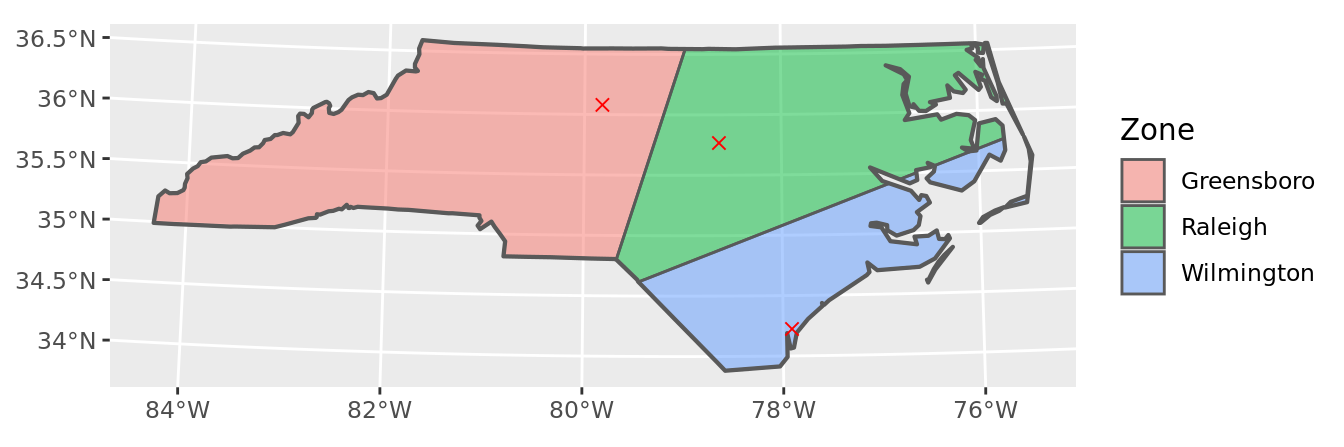

Making of a grid requires applying sf::st_make_grid() to the NC state with second argument of grid cell size – in our case 50 by 50 miles; the resulting object will again be a geometry without any data (object of class sfc).

It is then converted back to sf class, with city names re-attached. I am also creating a technical key based on row number, as I will need an unique identification of each polygon (i.e. grid cell) in later stages of our process.

# create the grid object
grid <- state %>% 
  st_make_grid(cellsize = c(50 * 5280, 50 * 5280)) %>% # 50 × 50 miles
  st_sf() %>% # from sfc to sf
  st_intersection(state) %>% # cut to shape of NC state
  st_join(points) %>% # get names back
  mutate(id = row_number()) # generate key for later use

# display the grid
ggplot() +
  geom_sf(data = grid, aes(fill = name), alpha = .5) +
  geom_sf(data = state, lwd = .75, fill = NA) + 
  geom_sf(data = points, color = "red", pch = 4, size = 2) +
  labs(fill = "Zone")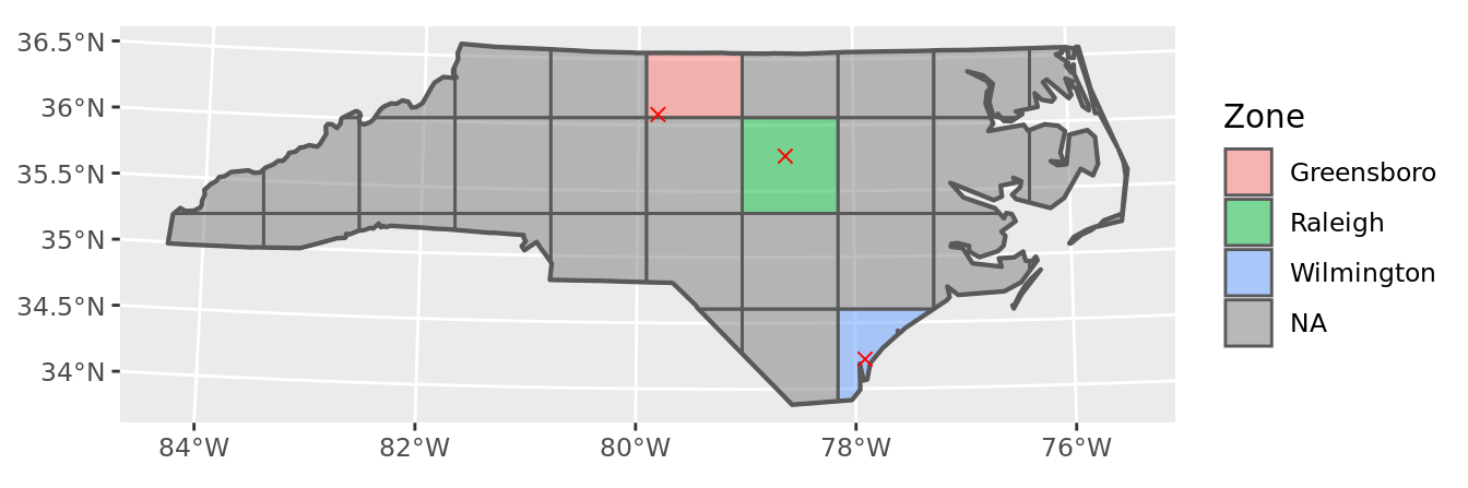

The third step is combining the county births data with geometries of interest via sf::st_intersection().

# naive intersection
buffers_raw <- buffers %>% 
  st_intersection(counties) # raw intersection

# this will not do for a result...
chart(buffers_raw)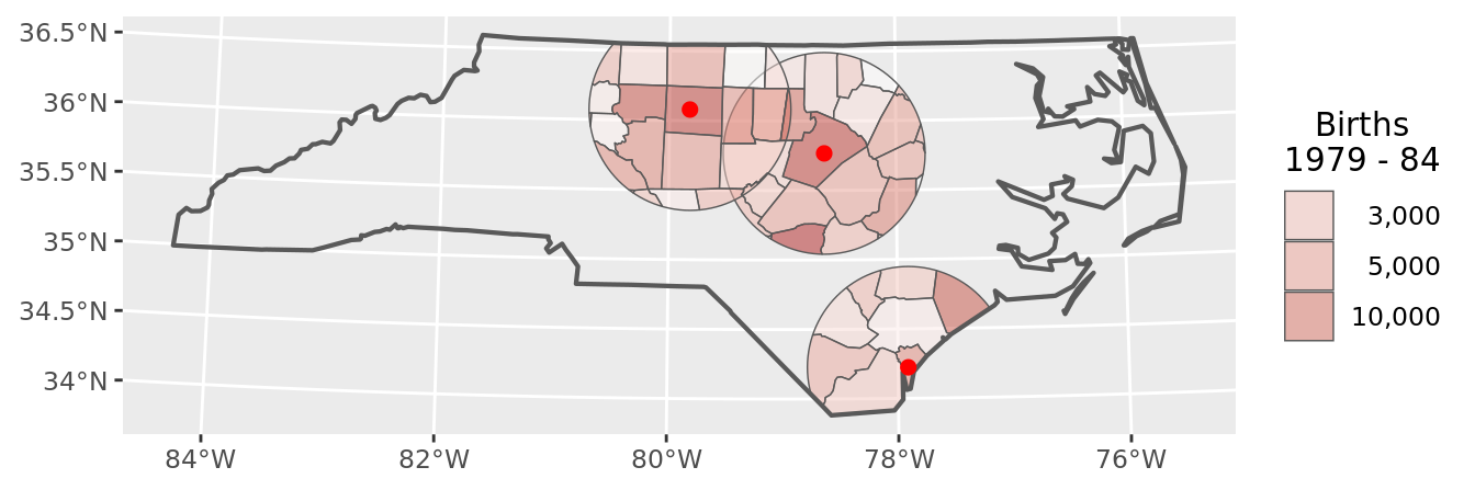

This obviously is not a satisfactory result, as the data retain the original county dimension.

It is necessary to dissolve the counties, and assign a proportion of the births measure to each buffer polygon; it is reasonable to assume an equal density of the births metric per county area, and based on that assign births to buffer in proportion of the county area contained in the buffer.

From technical perspective it is necessary to have two items in place before this step:

total area of source polygons (the intersection will split some county polygons, so the original area has to be calculated beforehand)
unique id of target polygon, which will serve as a grouping variable; for the buffers and Voronoi polygons city name is OK, for the grid a technical id is necessary

# new data object based on buffers
buffers_data <- buffers %>% 
  st_intersection(counties) %>% # raw intersection
  mutate(in_area = units::drop_units(st_area(.))) %>% # area of polygon
  # calculate a proportion of births equal to proportion of area
  mutate(BIR79 = BIR79 * in_area / cty_area) %>% 
  group_by(name) %>% # group by name of buffer
  summarise(BIR79 = sum(BIR79)) # total of births in named buffer

# plot the results
chart(buffers_data)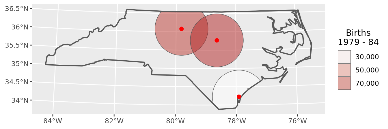

The technique to assign birth data to Voronoi polygons is exactly the same as for the spatial buffers.

# new data object based on Voronoi polygons
voronoi_data <- voronoi %>% 
  st_intersection(counties) %>% # raw intresection
  mutate(in_area = units::drop_units(st_area(.))) %>% # area of polygon
  # calculate a proportion of births equal to proportion of area
  mutate(BIR79 = BIR79 * in_area / cty_area) %>% 
  group_by(name) %>% # group by name of Voronoi polygon
  summarise(BIR79 = sum(BIR79)) # total of births in named polygon

# plot the results
chart(voronoi_data)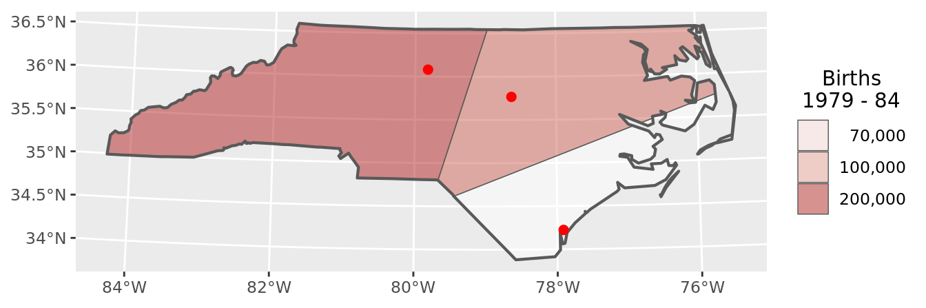

Two important differences between buffers and Voronoi polygons are that:

the Voronoi polygons are not overlapping
the Voronoi polygons cover the entire NC state

This has the consequence that we can confirm our result of our calculation by comparing the totals per county with totals per Voronoi polygons; we can reasonable expect these two to be equal (there is no double counting, and the entire state is covered).

# checksum - do the totals add up?
all.equal(sum(counties$BIR79), sum(voronoi_data$BIR79))

## [1] TRUE

Lastly we consider the grid cells.

The technique is again the same – assign to each grid cell a proportion of county births equal to the proportion of county area.

In this case the technical key of grid cells comes handy as grouping variable, as there are more grid cells than city points.

# new data object based on grid
grid_data <- grid %>% 
  st_intersection(counties) %>% # raw intersection
  mutate(in_area = units::drop_units(st_area(.))) %>% # area of cell
  # calculate a proportion of births equal to proportion of area
  mutate(BIR79 = BIR79 * in_area / cty_area) %>% 
  group_by(id) %>% # group by id of grid cell
  summarise(BIR79 = sum(BIR79)) # total of births in cell by id

# plot the results
chart(grid_data)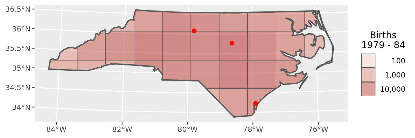

Again, as the cells (like the Voronoi polygons, and unlike the buffers) cover the entire area of NC state with zero overlap it makes sense to compare the totals.

# checksum - do the totals add up?
all.equal(sum(counties$BIR79), sum(grid_data$BIR79))

## [1] TRUE

The final step is considering which spatial aggregation technique is the most appropriate in your use case.

This is (obviously) impossible to determine without some understanding of your use case.

A few rules of thumb to consider are:

buffers are often a good idea when considering “bad” things – such as number of burglaries in the neighborhood; such metrics can spoil the figures for multiple areas of interest without diminishing.
Voronoi polygons are a good idea when considering “nice” things – such as potential customers, who will either visit store A or store B, but not both, for their shopping.
grid cells are good idea when you need to consider not only a presence of something, but also an absence of the thing – cells being empty carry information. Grid cells also create the illusion of impartiality – the entire region is covered, and even cells seem fair.