The “Napoleon in Russia” map by Charles Joseph Minard is a justly famous piece of 19th century infographic.

It has been a subject to many modern era re-visions and re-interpretations after being popularized by John Tukey. One of the re-creations was featured prominently in the original {ggplot2} article by you-know-who. One could be excused for considering the matter settled.
One approach that I have not seen before, however, is re-visioning the Minard’s map using actual geocoded data.
The usual way to drawing the map is to use a highly schematized approach, taking care to draw the incoming and outgoing armies separately - even though the army spent a significant part of the homeward march backtracking itself. This led to disastrous results, as the Grande Armée, in the accepted fashion of early modern armies, lived off the land coming in; there was little left to live off going out.
A complication I had to face was the somewhat dated French toponymy. The names that Monsieur Minard used in his map proved difficult to use in modern geocoding use cases.
This was due to a number of reasons:
- Lithuania has freed itself from the shackles of Polish rule, and Kowno and Wilna became Kaunas and Vilnius
- Gzhatsk (marked as Chjat in the original map) had its name changed in 1968 after an upstart major, who shot to fame from his birthplace nearby
- some Russian names are simply difficult; there is not much that can be done with Maloyaroslavets, or Malo-Jarosewii in the map. On the other hand the treatment that Vyazma received (becoming Wizma in Minard’s rendering and Wixma in Hadley’s) was somewhat surprising.
At the end I solved this with a little Wikipedia-fu. I am reasonably comfortable in reading Cyrillic, but I find it rather difficult to write it, given the cruel and unusual layout or the Russian keyboard.
I was able to place all the major map locations, with only minor difficulties:
- the path of the force led by Marshal Macdonald to lay siege to Riga ended up much more prominent than in the original map; also there was no way to make it appear to start in the same direction as the main army
- in order to make the path of the force led by Marshal Oudinot appear correctly crooked around Glubokoe (Gloubokoe) I had to include the unsuccessful siege of Dinaburg that was not among Minard’s original labels
- I was unsuccessful in geocoding Tarutino – labelled Tarantino, as in Quentin Tarantino, by Minard – as it has a naming conflict with a somewhat bigger city in Ukraine. As only a part of Napoleon’s forces was involved (the Emperor left Moscow only after this Russian victory) I chose to omit it entirely.
- instead of Studianka marked by Minard for the Berezina crossing I used nearby Borisov. It is close enough not to matter in our use case (it did matter to Napoleon, as he found the bridge in the town burned, and had to build his own nearby).
At the end I had a data frame of 29 locations (with a few necessary duplicites).
library(tidygeocoder)
library(ggplot2)
library(dplyr)

minard_raw <- data.frame(city = c("Kaunas", "Vilnius", "Глыбо́кае", "Витебск",
                                  "Смоленск", "Дорогобу́ж", "Гага́рин"  ,
                                  "Можа́йск",  "Москва", "Москва",
                                  "Малояросла́вец", "Можа́йск", "Вя́зьма",
                                  "Дорогобу́ж", "Смоленск", "О́рша",
                                  "Бобр", "Бори́сов",  "Маладзечна",
                                  "Сморгонь", "Vilnius", "Kaunas", # La Grande Armée
                                  "Vilnius", "Daugavpils",
                                  "По́лоцк", "Бобр", # reserve in Polotskt
                                  "Kaunas", "Riga",
                                  "Riga", "Kaunas"), # the siege of Riga
                     direction = c("outward", "outward", "outward", "outward",
                                   "outward", "outward", "outward", "outward",
                                   "outward", "homeward", "homeward", "homeward",
                                   "homeward", "homeward", "homeward", "homeward",
                                   "homeward", "homeward", "homeward", "homeward",
                                   "homeward", "homeward", # Napoleon
                                   "outward", "outward", "homeward",
                                   "homeward", # Oudinot
                                   "outward", "outward", "homeward",
                                   "homeward"), # MacDonald
                     strength = c(422000, 340000, 280000, 210000, 145000,
                                  140000, 127100, 100000, 100000, 100000,
                                  98000, 87000, 55000, 37000, 24000, 20000,
                                  50000, 28000, 12000, 14000, 8000,
                                  4000, # Napoleon
                                  60000, 40000, 33000, 28000, # Oudinot
                                  22000, 22000, 6000, 6000), # MacDonald
                     leader = c(rep("Napoleon", 22),
                                rep("Oudinot", 4),
                                rep("MacDonald", 4)))
For geocoding I used the highly recommended {tidygeocoder} package by Jesse Cambon.
It supports several backend engines and allows for multiple options to identify objects of interest: addresses, streets, cities, counties, states and so on.
In my use case the method “osm” (for OpenStreetMap backend) and selecting by city performed the best. It also made a rather concise three line call.
# let tidygeocoder perform its magic!
minard_geocoded <- minard_raw %>%
  tidygeocoder::geocode(city = city,
                        method = "osm")
Now that we have geocoded the raw data frame we can do a quick overview.
Note that the output from tidygeocoder::geocode() is still a regular data frame, and not the special {sf} kind. This will have implications in plotting the path, as we can use ggplot2::geom_path(), and not geom_sf() and friends.
knitr::kable(minard_geocoded,
             format.args = list(big.mark = ",",
scientific = FALSE))| city | direction | strength | leader | lat | long |
|---|---|---|---|---|---|
| Kaunas | outward | 422,000 | Napoleon | 54.89821 | 23.90448 |
| Vilnius | outward | 340,000 | Napoleon | 54.68705 | 25.28291 |
| Глыбо́кае | outward | 280,000 | Napoleon | 55.13923 | 27.68458 |
| Витебск | outward | 210,000 | Napoleon | 55.19302 | 30.20704 |
| Смоленск | outward | 145,000 | Napoleon | 54.77897 | 32.04718 |
| Дорогобу́ж | outward | 140,000 | Napoleon | 54.91482 | 33.29891 |
| Гага́рин | outward | 127,100 | Napoleon | 55.55339 | 34.99051 |
| Можа́йск | outward | 100,000 | Napoleon | 55.50648 | 36.02131 |
| Москва | outward | 100,000 | Napoleon | 55.75054 | 37.61748 |
| Москва | homeward | 100,000 | Napoleon | 55.75054 | 37.61748 |
| Малояросла́вец | homeward | 98,000 | Napoleon | 55.01218 | 36.45902 |
| Можа́йск | homeward | 87,000 | Napoleon | 55.50648 | 36.02131 |
| Вя́зьма | homeward | 55,000 | Napoleon | 55.21036 | 34.29952 |
| Дорогобу́ж | homeward | 37,000 | Napoleon | 54.91482 | 33.29891 |
| Смоленск | homeward | 24,000 | Napoleon | 54.77897 | 32.04718 |
| О́рша | homeward | 20,000 | Napoleon | 54.51190 | 30.42545 |
| Бобр | homeward | 50,000 | Napoleon | 54.34169 | 29.27448 |
| Бори́сов | homeward | 28,000 | Napoleon | 54.22407 | 28.51178 |
| Маладзечна | homeward | 12,000 | Napoleon | 54.30733 | 26.83891 |
| Сморгонь | homeward | 14,000 | Napoleon | 54.48178 | 26.40128 |
| Vilnius | homeward | 8,000 | Napoleon | 54.68705 | 25.28291 |
| Kaunas | homeward | 4,000 | Napoleon | 54.89821 | 23.90448 |
| Vilnius | outward | 60,000 | Oudinot | 54.68705 | 25.28291 |
| Daugavpils | outward | 40,000 | Oudinot | 55.87123 | 26.51593 |
| По́лоцк | homeward | 33,000 | Oudinot | 55.48547 | 28.76823 |
| Бобр | homeward | 28,000 | Oudinot | 54.34169 | 29.27448 |
| Kaunas | outward | 22,000 | MacDonald | 54.89821 | 23.90448 |
| Riga | outward | 22,000 | MacDonald | 56.94940 | 24.10518 |
| Riga | homeward | 6,000 | MacDonald | 56.94940 | 24.10518 |
| Kaunas | homeward | 6,000 | MacDonald | 54.89821 | 23.90448 |
Before plotting we need to create two helper objects:
- data frame of city labels, with duplicities removed
- a helper of X and Y offsets for labels; I wish there was a reliable automatic way to place the labels, but at the end I had to resort to manual adjustments
# city labels
city_labels <- minard_geocoded %>%
  select(city, lat, long) %>%
  distinct()

# offsets - a kludge to make the labels legible
kludge <- data.frame(horizontal = c(0, -.25, -.2, 0, 0,
                                    .25, -.5, 0, 0, 0,
                                    .4, .25, .4, -.2, -.2,
                                    .7, -.25, .4, 0),
                     vertical = c(-.2, -.2, .3, .3, -.3,
                                  -.3, .2, .2, .2, -.2,
                                  -.3, -.2, -.15, .2, -.15,
                                  .1, .2, .2, .15))
Now we can proceed to drawing the map itself. The logic of its construction follows in principle the ggplot2 article, with only minor differences – I have changed the order of the groups, so that advancing Napoleon gets drawn over retreating Oudinot, as in the original map, and of course all the cities are in their proper places.
# and finally, the plot itself
ggplot() +
  # paths taken by the armies
  geom_path(data = minard_geocoded,
            aes(x = long,
                y = lat,
                size = strength,
                color = direction,
                # make sure Napoleon gets drawn over Oudinot, not the other way round
                group = factor(leader, levels = c("Oudinot",
                                                  "MacDonald",
                                                  "Napoleon")))) +
  # labels for the cities
  geom_text(data = city_labels,
            aes(x = long,
                y = lat,
                label = city),
            family = "Old Standard TT", # an old fashioned Cyrillic font
            fontface = "italic",
            # I wish that this was not necessary...
            nudge_x = kludge$horizontal,
            nudge_y = kludge$vertical) +
  scale_colour_manual(values = c("gray10",
                                 "#e8cbac")) + # the color Minard calls "rouge"
  scale_size(range = c(1/10, 17)) + # a "slight" exaggeration
  guides(color = F, size = F) + theme_void() + # just say "no" to distractions
  labs(title = "1812, or There and Back Again",
       subtitle = "geocoding the Minard's map") +
  theme(plot.title = element_text(hjust = 1/2,
                                  face = "bold"),
        plot.subtitle = element_text(hjust = 1/2,
                                     face = "italic"))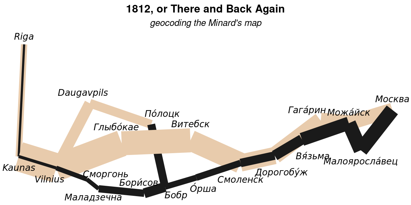
An alternative rendition of the map is over a basemap. Note how closely the path of the armies to Moscow follows current roads – the Smolensk road coming in, and the Kaluga road trying to break out (with the fateful decision to backtrack to Smolensk after Maloyaroslavets).
library(ggmap)

# a basemap / consider maptype = "terrain-background" for an alternative look
basemap <- get_stadiamap(bbox = c(left =  23,
                                  bottom = 53.75,
                                  right = 39.25,
                                  top = 57.15),
                         maptype = "stamen_toner",
                         zoom = 7)

# the plot again, without text labels this time
ggmap(basemap) +
 geom_path(data = minard_geocoded,
            aes(x = long,
                y = lat,
                size = strength,
                color = direction,
                group = factor(leader, levels = c("Oudinot",
                                                  "MacDonald",
                                                  "Napoleon"))),
           alpha = 2/3) + # a slight alpha to retain a hint of the basemap
  scale_colour_manual(values = c("gray10",
                                 "#e8cbac")) +
  scale_size(range = c(1/4, 17)) +
  guides(color = F, size = F) +
  theme_void() +
  labs(title = "1812, or There and Back Again",
       subtitle = "geocoding the Minard's map") +
  theme(plot.title = element_text(hjust = 1/2,
                                  face = "bold"),
        plot.subtitle = element_text(hjust = 1/2,
                                     face = "italic"))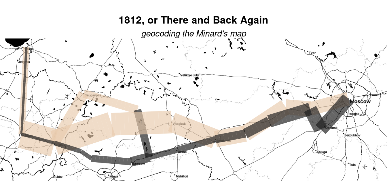
Yet another alternative approach is presenting the Minard’s map interactively via {leaflet} and leaflet.js.
This will take some effort, as it is necessary to first translate the army path from a sequence of lat-lon points to a spatial lines object. This needs to be done segment by segment, to preserve the troops information, and care must be taken to maintain the three separate forces.
Once the lines object is in place the leaflet call itself is not a difficult one to make.
library(sf)

# first make the data frame spatial object
sf_path <- minard_geocoded %>%
  st_as_sf(coords = c("long", "lat"), crs = 4326) %>%
  mutate(direction = as.factor(direction)) # factor for color palette assignment

minard_lines <- NULL # initiate an empty object

for (captain in unique(sf_path$leader)) { # i.e. Napoleon, Oudinot, MacDonald

  wrk_army <- subset(sf_path, leader == captain)

  # cycle over all segments, except the last one
  for (i in 1:(nrow(wrk_army)-1)) {

    # line object from two points
    wrk_line  <- wrk_army[c(i, i+1), ] %>% # current & next point coords
      st_coordinates() %>%
      st_linestring() %>%
      st_sfc()

    # a single row of results dataframe
    line_data <- data.frame(
      direction = wrk_army$direction[i],
      strength = wrk_army$strength[i],
      leader = wrk_army$leader[i],
      label = paste0(wrk_army$city[i], " to ",
                     wrk_army$city[i+1], "<br>army strength ",
                     format(wrk_army$strength[i],
                            big.mark = ",",
                            scientific = F), " men."),
      geometry = wrk_line
    )

    # bind the single row to the output object
    if (is.null(minard_lines)) {

      minard_lines <- line_data

    } else {
      minard_lines <- dplyr::bind_rows(minard_lines,
                                       line_data)

    } # /if - binding results

  } # /for segment

} # /for leader

# finalize the linear object
minard_lines <- st_as_sf(minard_lines, crs = 4326)

library(leaflet)

# palette for direction
pal <- colorFactor(c("gray10", "#e8cbac"),
                   minard_lines$direction)

# the map itself
leaflet(data = minard_lines) %>%
  addProviderTiles("CartoDB.Positron") %>%
  addPolylines(weight = ~strength/15000,
               color = ~pal(direction),
               opacity = 1,
               popup = ~label)
I suppose I could end here, having demonstrated the possibility of geocoding the Minard’s map locations (after some necessary adjustments).
But there is another interesting aspect of the 1812 campaign that I discovered when doing research for this blog post that I would like to share here:
The French tradition gives strong accent to hardship caused by winter cold – look at the prominence of the temperature data in the original map. In this way the defeat can be explained away as due to forces of Nature, or Fate, rather than enemy action.
The Russian tradition takes issue with that – it goes like “Sure, there was some snow, what would you expect in winter? But nothing really harsh, just look at the Berezina river; it was not even frozen over, don’t you see??” and instead attributes the French losses to starvation caused by marching over countryside they themselves plundered when coming in. This makes them seem kind of self inflicted.
Also notable is how the Russian tradition stresses the “ordinary people” aspect – 1812 being the original Patriotic War – and downplays the role of senior officers (other than Kutuzov and Bagration).
This may, and may not, relate to the fact that many of the generals on the Russian side were ethnic Germans. Fun fact here: Tsar Alexander employed in his staff a certain von Clausewitz, who played a key role in negotiating the betrayal of Napoleon by Ludwig Yorck, commander of the Prussian auxiliary corps at Riga.