Merging Geometry of {sf} Objects in R

A frequent use case in spatial data processing is merging multiple geometries. In my line of work this usually involves merging polygons of administrative regions to larger, seemingly arbitrary, units – sales areas and what not.

In the olden days of {sp}, when shapefiles were S3 objects sui generis, this was not exactly easy. Now, with the {sf} package, when spatial objects are modified data.frames (and data.frame manipulation is supported by the mighty {dplyr}) this process is much less challenging.

In fact it is so easy it might seem like magic.

To demonstrate the workflow I am using the North Carolina shapefile from the {sf} package, and a data frame of three semi random cities.

To make the process more fun (for an European, metric born & raised) I am projecting the data to a quaint local CRS denominated in US survey feet.

library(sf)
library(dplyr)
library(ggplot2)

# NC counties as polygons - a shapefile shipped with the sf package
counties <- st_read(system.file("shape/nc.shp", package = "sf"), quiet = T) %>% 
  st_transform(2264) # a feety CRS, to make it interesting :)

# three NC cities as points
points <- data.frame(name = c("Raleigh", "Greensboro", "Wilmington"),
                     x = c(-78.633333, -79.819444, -77.912222),
                     y = c(35.766667, 36.08, 34.223333)) %>% 
  st_as_sf(coords = c("x", "y"), crs = 4326) %>% 
  st_transform(2264) # transform to a feety CRS


# buffer of 50 miles around Raleigh city centre
buffer <- st_buffer(subset(points, name == "Raleigh"), 5280 * 50)

First a simple overview of my spatial objects:

100 counties of North Carolina
3 cities in NC as points
a red buffer of 50 miles around Raleigh (the state capital)

ggplot() +
  geom_sf(data = counties) +
  geom_sf(data = points, aes(color = name), show.legend = "point") +
  geom_sf(data = buffer, fill = NA, color = "red") +
  scale_color_viridis_d() +
  theme(legend.position = "bottom") +
  labs(color = "City name:")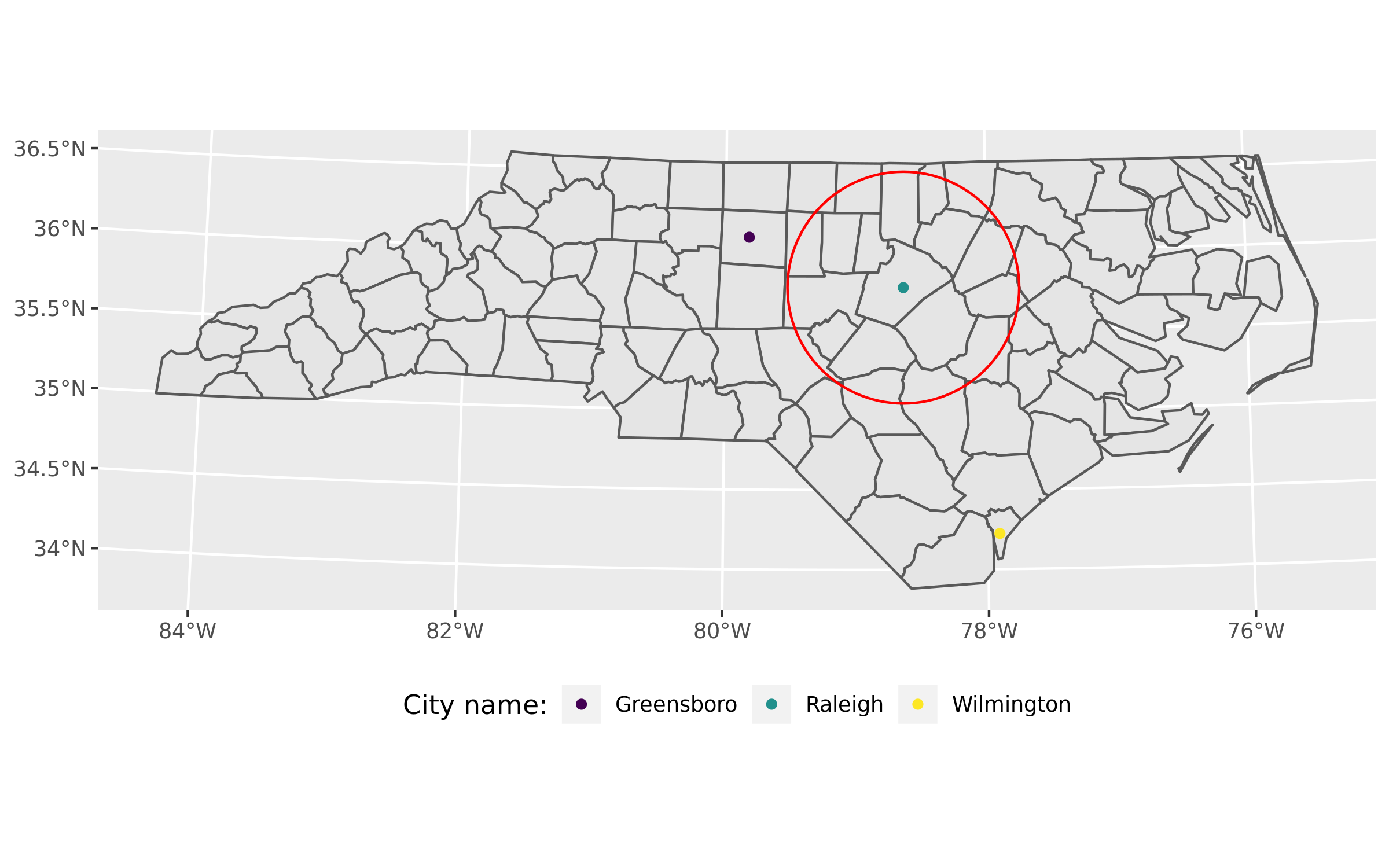

The first step is determining which counties are at least partly covered by the red buffer.

The best way to handle this is via sf::st_intersects() and setting the sparse argument to false (so a logical vector will be returned).

In this case the logical vector is recoded to “yes” / “no” string values via ifelse().

counties$close2raleigh <- ifelse(sf::st_intersects(counties, buffer, sparse = F), 
                                 "Yes", 
                                 "No")

glimpse(counties)

## Observations: 100
## Variables: 16
## $ AREA          <dbl> 0.114, 0.061, 0.143, 0.070, 0.153, 0.097, 0.062, 0…
## $ PERIMETER     <dbl> 1.442, 1.231, 1.630, 2.968, 2.206, 1.670, 1.547, 1…
## $ CNTY_         <dbl> 1825, 1827, 1828, 1831, 1832, 1833, 1834, 1835, 18…
## $ CNTY_ID       <dbl> 1825, 1827, 1828, 1831, 1832, 1833, 1834, 1835, 18…
## $ NAME          <fct> Ashe, Alleghany, Surry, Currituck, Northampton, He…
## $ FIPS          <fct> 37009, 37005, 37171, 37053, 37131, 37091, 37029, 3…
## $ FIPSNO        <dbl> 37009, 37005, 37171, 37053, 37131, 37091, 37029, 3…
## $ CRESS_ID      <int> 5, 3, 86, 27, 66, 46, 15, 37, 93, 85, 17, 79, 39, …
## $ BIR74         <dbl> 1091, 487, 3188, 508, 1421, 1452, 286, 420, 968, 1…
## $ SID74         <dbl> 1, 0, 5, 1, 9, 7, 0, 0, 4, 1, 2, 16, 4, 4, 4, 18, …
## $ NWBIR74       <dbl> 10, 10, 208, 123, 1066, 954, 115, 254, 748, 160, 5…
## $ BIR79         <dbl> 1364, 542, 3616, 830, 1606, 1838, 350, 594, 1190, …
## $ SID79         <dbl> 0, 3, 6, 2, 3, 5, 2, 2, 2, 5, 2, 5, 4, 4, 6, 17, 4…
## $ NWBIR79       <dbl> 19, 12, 260, 145, 1197, 1237, 139, 371, 844, 176, …
## $ geometry      <MULTIPOLYGON [US_survey_foot]> MULTIPOLYGON (((1270814 …
## $ close2raleigh <chr[,1]> "No", "No", "No", "No", "No", "No", "No", "No"…

The dataset now has 100 observations (counties) with 16 variables (including the special geometry column).

Of the 100 counties in NC there are 25 that are at least partly covered by the 50 mile buffer around Raleigh.

ggplot() +
  geom_sf(data = counties, aes(fill = close2raleigh)) +
  geom_sf(data = subset(points, name == "Raleigh"), pch = 4, color = "red") +
  geom_sf(data = buffer, fill = NA, color = "red") +
  scale_fill_viridis_d() +
  theme(legend.position = "bottom") +
  labs(fill = "Close to Raleigh?")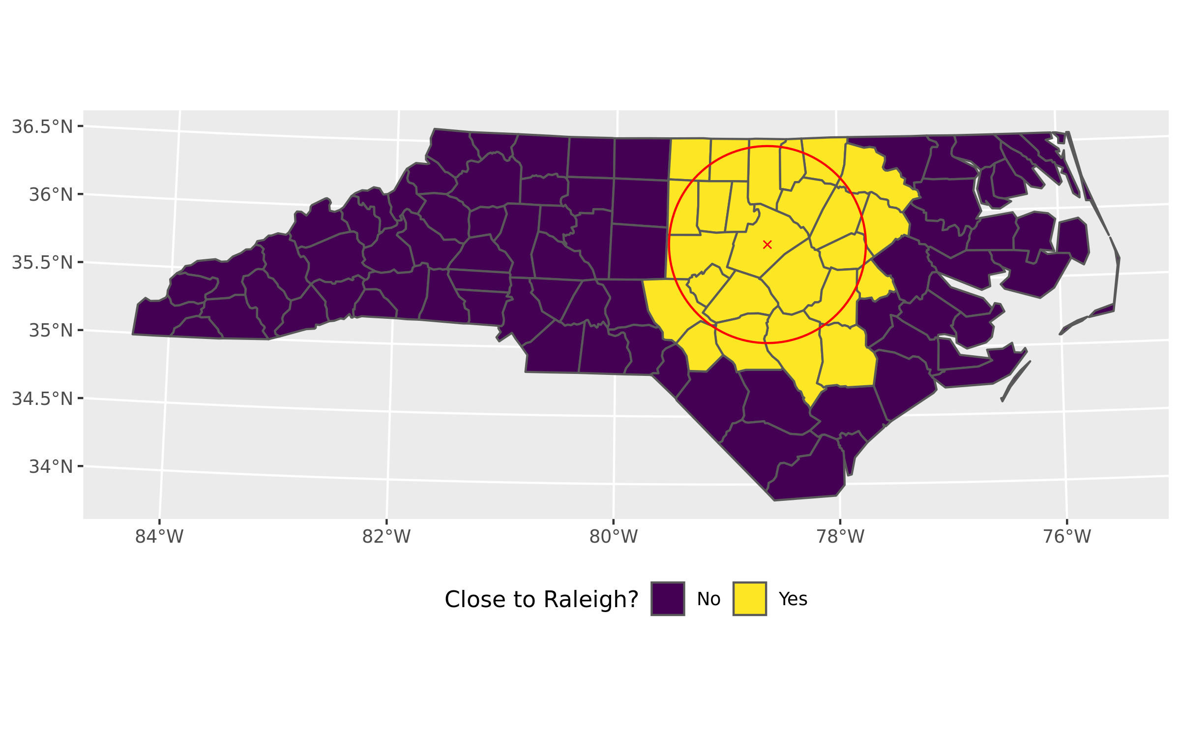

The “magic” part of merging the counties according to the value of close2raleigh column is straightforward – performing a dplyr::group_by() followed by dplyr::summarize().

In many cases it would be advantageous to perform some additional calculations, such as summarizing population or customer potential of the areas; in this example I have omitted this for the sake of clarity and focused on the merging operation only.

counties <- counties %>% 
  group_by(close2raleigh) %>% 
  summarise()

glimpse(counties)

## Observations: 2
## Variables: 2
## $ close2raleigh <chr> "No", "Yes"
## $ geometry      <GEOMETRY [US_survey_foot]> MULTIPOLYGON (((2739147 314.…

The merged dataset now has only two variables – the close2raleigh grouping variable, plus the special geometry column. It has two observations, one for each “yes” and “no” value of close2raleigh.

ggplot() +
  geom_sf(data = counties, aes(fill = close2raleigh)) +
  geom_sf(data = subset(points, name == "Raleigh"), pch = 4, color = "red") +
  geom_sf(data = buffer, fill = NA, color = "red") +
  scale_fill_viridis_d() +
  theme(legend.position = "bottom") +
  labs(fill = "Close to Raleigh?")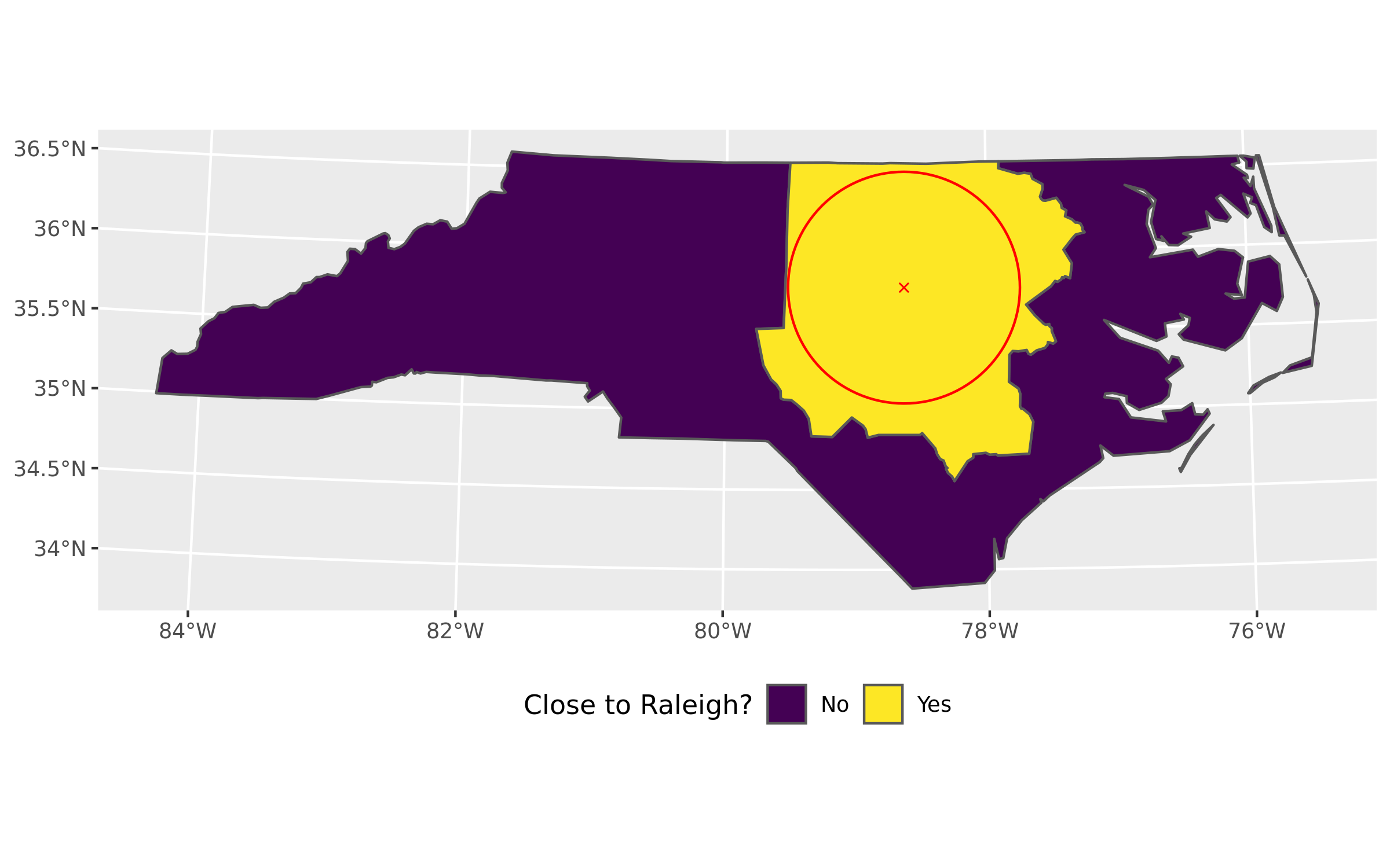

A basic understanding of dplyr data manipulation is by now common. On the other hand the application of the dplyr verbs to spatial data science workflow is not that well discussed, and in my opinion an interesting simplification in a number of use cases.