A question was raised recently on the RStudio discussion forum about an algorithm for linking spatial points by a network of lines.
The lines from points use case is frequently utilized in both visualizing of regional development – the lines representing flow from one region to another via color and / or thickness – and in network analysis – measuring & visualizing distance (i.e. length of the line) – between two or more areas of interest.
As I was unable to refer the poster of the question to a suitable published walkthrough I propose one of my own.
It is based on a function (I might be able to extend it into a package when time allows) points_to_lines(). The function takes four arguments, three of which are mandatory:
data frame of spatial points, expected in
{sf}package format; it is placed as the first argument, so the function is pipe friendlyname of column containing technical IDs of points (typically FIPS codes in the US, NUTS in the EU, or some other ID)
name of column containing names of the points for labels
indication whether order of the points matters (meaning whether line from A to B is equivalent to line from B to A); default is
TRUE
The function returns a spatial data frame of four columns: ID of starting point, ID of ending point, label (names of the two points, separated by a dash) and a geometry column of type LINESTRING; the geometry will be in the same CRS as original points.
library(sf)
library(dplyr)

points_to_lines <- function(data, ids, names, order_matters = TRUE) {

  # dataframe of combinations - based on row index
  idx <- expand.grid(start = seq(1, nrow(data), 1),
                     end = seq(1, nrow(data), 1)) %>%
    # no line with start & end being the same point
    dplyr::filter(start != end) %>%
    # when order doesn't matter just one direction is enough
    dplyr::filter(order_matters | start > end)


  # cycle over the combinations
  for (i in seq_along(idx$start)) {

    # line object from two points
    wrk_line  <- data[c(idx$start[i], idx$end[i]), ] %>%
      st_coordinates() %>%
      st_linestring() %>%
      st_sfc()

    # a single row of results dataframe
    line_data <- data.frame(
      start = pull(data, ids)[idx$start[i]],
      end = pull(data, ids)[idx$end[i]],
      label = paste(pull(data, names)[idx$start[i]],
                    "-",
                    pull(data, names)[idx$end[i]]),
      geometry = wrk_line
    )

    # bind results rows to a single object
    if (i == 1) {
      res <- line_data

    } else {
      res <- dplyr::bind_rows(res, line_data)

    } # /if - saving results

  } # /for

  # finalize function result
  res <- sf::st_as_sf(res, crs = sf::st_crs(data))

  res

} # /function
The function can be easily sourced & then used as a one liner in any script; it requires only {sf} and {dplyr} packages, so no cruel or unusual dependencies are involved.
The intended use case is to generate a spatial data frame of lines from a spatial data frame of points (either centroids or points-on-a-surfaces or what not) and the result then joined with actual data via one of the dplyr::*_join() functions.
To demonstrate the use of the function I am showing links between five semi random counties in North Carolina (using the popular nc.shp shapefile that ships with the {sf} package, and is therefore widely available).
# Well known & much loved shapefile of NC included with sf package
nc_polygons <- sf::st_read(system.file("shape/nc.shp", package="sf"), quiet = T)

set.seed(16)

# five semi random county centroids
nc_points <- nc_polygons %>%
  sf::st_centroid() %>%
  slice(sample(1:nrow(nc_polygons), 5))

# function of lines from points
nc_lines <- points_to_lines(nc_points, ids = "FIPS", names = "NAME")

# a graphic overview
library(ggplot2)
ggplot() +
  geom_sf(data = nc_polygons, color = "gray45", fill = NA) +
geom_sf(data = nc_lines, color = "red") 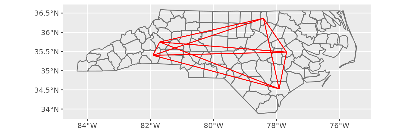
The algorithm to create lines comes in two flavors, depending on whether order matters for your use case.
In case order does matter – i.e. a line from Greene to Pender counties is different from the one from Pender to Greene – there will be nrow(data) × (nrow(data) - 1) lines (each point is connected to every other point except itself).
In case order does not matter – i.e. once a line is drawn from Greene to Pender there will be no need to plot another in opposite direction – there will be only half as much lines required.
To pick which behavior is desirable change the value of order_matters argument; the default is TRUE, meaning yes, order does matter.
# when order matters >> both directions are required >> 20 rows
points_to_lines(nc_points, ids = "FIPS", names = "NAME", order_matters = T) %>%
knitr::kable()| start | end | label | geometry |
|---|---|---|---|
| 37079 | 37141 | Greene - Pender | LINESTRING (-77.67889 35.48… |
| 37161 | 37141 | Rutherford - Pender | LINESTRING (-81.91787 35.39… |
| 37181 | 37141 | Vance - Pender | LINESTRING (-78.41127 36.36… |
| 37023 | 37141 | Burke - Pender | LINESTRING (-81.70216 35.74… |
| 37141 | 37079 | Pender - Greene | LINESTRING (-77.91628 34.52… |
| 37161 | 37079 | Rutherford - Greene | LINESTRING (-81.91787 35.39… |
| 37181 | 37079 | Vance - Greene | LINESTRING (-78.41127 36.36… |
| 37023 | 37079 | Burke - Greene | LINESTRING (-81.70216 35.74… |
| 37141 | 37161 | Pender - Rutherford | LINESTRING (-77.91628 34.52… |
| 37079 | 37161 | Greene - Rutherford | LINESTRING (-77.67889 35.48… |
| 37181 | 37161 | Vance - Rutherford | LINESTRING (-78.41127 36.36… |
| 37023 | 37161 | Burke - Rutherford | LINESTRING (-81.70216 35.74… |
| 37141 | 37181 | Pender - Vance | LINESTRING (-77.91628 34.52… |
| 37079 | 37181 | Greene - Vance | LINESTRING (-77.67889 35.48… |
| 37161 | 37181 | Rutherford - Vance | LINESTRING (-81.91787 35.39… |
| 37023 | 37181 | Burke - Vance | LINESTRING (-81.70216 35.74… |
| 37141 | 37023 | Pender - Burke | LINESTRING (-77.91628 34.52… |
| 37079 | 37023 | Greene - Burke | LINESTRING (-77.67889 35.48… |
| 37161 | 37023 | Rutherford - Burke | LINESTRING (-81.91787 35.39… |
| 37181 | 37023 | Vance - Burke | LINESTRING (-78.41127 36.36… |
# if directions don't matter >> a single direction is enough >> 10 rows only
points_to_lines(nc_points, ids = "FIPS", names = "NAME", order_matters = F) %>%
knitr::kable()| start | end | label | geometry |
|---|---|---|---|
| 37079 | 37141 | Greene - Pender | LINESTRING (-77.67889 35.48… |
| 37161 | 37141 | Rutherford - Pender | LINESTRING (-81.91787 35.39… |
| 37181 | 37141 | Vance - Pender | LINESTRING (-78.41127 36.36… |
| 37023 | 37141 | Burke - Pender | LINESTRING (-81.70216 35.74… |
| 37161 | 37079 | Rutherford - Greene | LINESTRING (-81.91787 35.39… |
| 37181 | 37079 | Vance - Greene | LINESTRING (-78.41127 36.36… |
| 37023 | 37079 | Burke - Greene | LINESTRING (-81.70216 35.74… |
| 37181 | 37161 | Vance - Rutherford | LINESTRING (-78.41127 36.36… |
| 37023 | 37161 | Burke - Rutherford | LINESTRING (-81.70216 35.74… |
| 37023 | 37181 | Burke - Vance | LINESTRING (-81.70216 35.74… |