Creating new polygons by dissolving borders of existing ones is a common use case - especially so when working in a sales environment, where sales areas frequently combine lower level units in a seemingly arbitrary fashion.
In this walkthrough I would like to share the process in a workflow I built on the sf package.
For my example I decided to split the shapefile of the city of Prague into two areas - the center and the outskirts based on a shapefile containing the 57 inner neighbourhoods.
The shapefile for Prague is from my package RCzechia (available on GitHub, but not really necessary - the technique will work with any shapefile), the other packages are the usual suspects for tidy and spatial work.
library(sf)
library(tidyverse)
library(RCzechia) # for the shapefile of Prague; available on CRAN
library(ggmap) # for geocoding
library(tmap) # for drawing charts

krovak <- 5514
# the official Czech CRS - with meters as units; necessary to calculate buffers ¨
# (WGS84 is in decimal degrees)

frmPraha <- casti() %>% # read in all city neigbouhrhoods
  filter(NAZ_OBEC == "Praha") %>% # select the 57 relevant to Prague
  st_transform(crs = krovak) # convert CRS from WGS84 to the metric one
For calculating the central parts I needed to determine the geographical center of Prague. Partly for personal reasons, and partly out of desire to see Google sweat, I chose the statue of Winston Churchill standing in front of the Prague School of Economics - hello, Alma Mater!
As for the definition of “central parts” of Prague I decided that any city neighbourhood that intesects a 5 kilometers circle around the statue of sir Winston is a part of the city center. And one that does not is not.
Note that I am using a coordinate reference system different from the usual WGS84 - the reason is that I will be working with buffers, and buffers do not enjoy working with decimal degrees (the unit of WGS84). It is better to transform to another CRS (and remember there is always a way back).
winston <- geocode("socha winstona churchilla praha", output = "latlon") %>%
  # lat long position of the statue of sir Winston, as data.frame
  # a word of warning - for ggmap::geocode() to work a Google API
  # has to be set up - see ?register_google for details
  st_as_sf(coords = c("lon", "lat"), crs = 4326) %>%
  # convert from data.frame to sf object, crs = WGS84
  st_transform(crs = krovak) # crs to the Czech metric one

bublina <- st_buffer(winston, dist = 5000)
# set buffer 5 kilometers around sir Winston
To calculate the intersection of the five kilometer buffer around sir Winston and the 57 city neighbourhoods I used the st_intersects() function. I found it important to use the sparse = F setting, as it forces the function to return a vector that can be put back in the data frame.
frmPraha$centrum <- st_intersects(frmPraha, bublina, sparse = F)
# new column; boolean value for in buffer / out of buffer; the sparse = F is important
# otherwise the result would be a list
# now a simple chart
tm_shape(frmPraha) + tm_borders(col = "grey40") + tm_fill(col = "centrum") +
tm_shape(winston) + tm_dots(size = 1/3, col = "red", shape = 4) + # sir Winston
tm_shape(bublina) + tm_borders(col = "red") # the 5 km bubble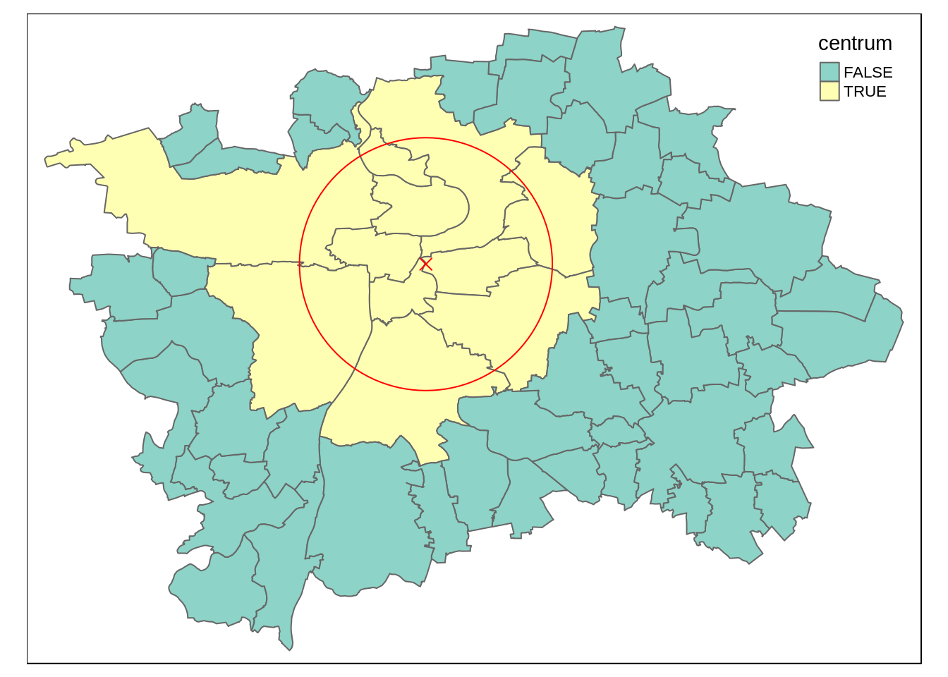 Now that I have a rough idea what the end result should look like comes the time for actual work. It will consist of three parts:
- dissolving the inner polygon (the center)
- dissolving the outer polygon (the outskirts)
- joining the center and outskirts back to one
sfdata frame
One important hack that I learned is to extend (buffer) the borders of the city neigbourhoods by half a meter.
This does not have a visible impact on the outcome (Prague is tens of kilometers long and wide, so half a meter makes no difference either way) but it helps to avoid artifacts (slivers) in place of former inner boundaries. It is a common problem with GEOS and one surprisingly hard to troubleshoot. The st_buffer() of half a meter dispenses of it elegantly.
The st_union() function returns just plain geometry, which is in sf terminology is a sfc object - a list containing geometry - and requires a call of st_sf() to become a data frame capable of holding additional data.
center <- frmPraha[frmPraha$centrum == T, ] %>% # select the central parts
  st_buffer(0.5) %>% # make a buffer of half a meter around all parts (to avoid slivers)
  st_union() %>% # unite to a geometry object
  st_sf() %>% # make the geometry a data frame object
  mutate(centrum = T) # return back the data value

outskirts <- frmPraha[frmPraha$centrum == F, ] %>% # select the non-central parts
  st_buffer(0.5) %>% # make a buffer of half a meter around all parts (to avoid slivers)
  st_union() %>% # unite to a geometry object
  st_sf() %>% # make the geometry a data frame object
  mutate(centrum = F) # return back the data value

frmPraha2 <- rbind(center,
                   outskirts) # merge central and non-central part to a single data frame
With the center and outskirts polygons bound back to a single sf data frame there is only one step left: to verify the results by drawing a map of the outcome.
tm_shape(frmPraha2) + tm_borders(col = "grey40") + tm_fill(col  = "centrum") +
  tm_shape(winston) + tm_dots(size = 1/3, col = "red", shape = 4) + # sir Winston
  tm_shape(bublina) + tm_borders(col = "red") # the 5 km bubble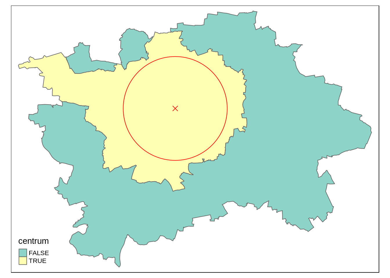
str(frmPraha2)## Classes 'sf' and 'data.frame': 2 obs. of 2 variables:
## $ centrum : logi TRUE FALSE
## $ geometry:sfc_GEOMETRY of length 2; first list element: List of 1
## ..$ : num [1:11845, 1:2] -738336 -738357 -738363 -738368 -738378 ...
## ..- attr(*, "class")= chr "XY" "POLYGON" "sfg"
## - attr(*, "sf_column")= chr "geometry"
## - attr(*, "agr")= Factor w/ 3 levels "constant","aggregate",..: NA
## ..- attr(*, "names")= chr "centrum"Lo and behold - a sf data frame with just two rows, one for center and one for the outskirts.
And while it was not my original intention the outskirts area is a single spatial object consisting of three separate polygons. Which I found rather neat.