In the Czech Republic it is common knowledge that the price of oil is the highest on the D1 highway, connecting Prague to Brno (the #1 and #2 Czech cities).
But as the saying goes in God we trust, all others bring data, and so I decided to test the common knowledge against real data. After all the “common knowledge” is commonly known to be fallible.
It turned out to be a project involving (chiefly) three packages:
- scraping of internet pages via rvest
- data vizualization via tmap
- shapefile of Czech Republic via RCzechia
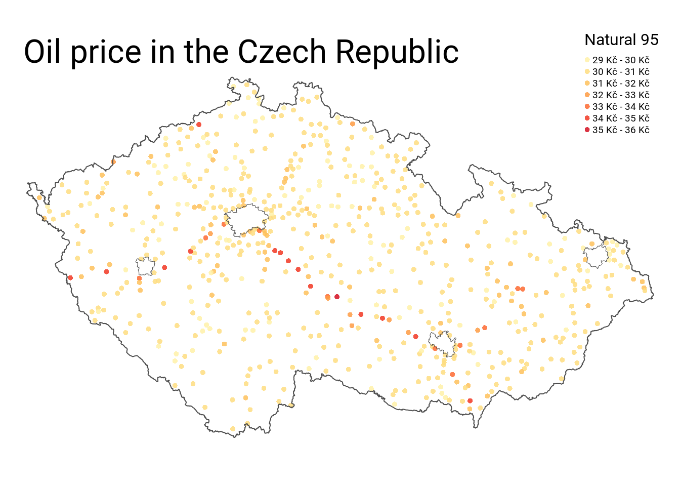
I obtained the average price of unleaded gasoline in 653 Czech towns (out of the 6 258 total recognized municipalities) by scraping web pages of Rádio Impulz. The data is current to 19.01.2018.
At the end the common knowledge turned to be rather accurate, and the shape of D1 highway connecting Prague and Brno pretty much jumps out of the plot.
What I did not expect, but what the data shows beyond doubt, is that the price of gasoline on D5 highway, going from Prague westwards to Pilsen and on to Munich, gives a fair fight to the infamous D1.
The code to generate the map is following:
# Initialization ----
library(rvest)
library(tmap)
library(tmaptools)
library(raster)
library(RCzechia) # set of shapefiles for the Czech Republic - devtools::install_github("jlacko/RCzechia")
library(stringr)
library(dplyr)
library(RColorBrewer)

url <- "http://benzin.impuls.cz/benzin.aspx?strana=" # url without page no.
frmBenzin <- data.frame() # empty data frame for data

bbox <- extent(republika) # a little more space around - enough for title and legend
bbox@ymax <- bbox@ymax + 0.35
bbox@ymin <- bbox@ymin - 0.15

# Scraping data ----

for (i in 1:56) { # Scrape data, translate and append to results

  impuls <- read_html(paste(url, i, sep = ''), encoding = "windows-1250")
  asdf <- impuls %>%
    html_table()

  frmBenzin <- rbind(frmBenzin, asdf[[1]])
}

# Cleaning data ----

frmBenzin$X1 <- NULL
colnames(frmBenzin) <- c("nazev", "obec", "okres","smes", "datum", "cena")
frmBenzin$cena <- gsub("(*UCP)\\s*Kč", "", frmBenzin$cena, perl = T) # regex is tricky - perl is safer
frmBenzin$cena <- as.double(frmBenzin$cena)
frmBenzin$datum <- as.Date(frmBenzin$datum, "%d. %m. %Y")
frmBenzin$okres <- gsub("Hlavní město\\s","",frmBenzin$okres)
frmBenzin$obec <- str_split(frmBenzin$obec, ",", simplify = T)[,1]
frmBenzin$key <- paste(frmBenzin$obec, frmBenzin$okres, sep = "/")

# Data wrangling ----

frmBenzinKey <- frmBenzin %>%
  select(key, cena, smes) %>%
  filter(smes == "natural95") %>% # only gasoline - no diesel
  group_by(key) %>%
  summarise(cena = mean(cena)) # average price in town

obce <- obce_body # from package RCzechia

obce$key <- paste(obce$Obec, obce$Okres, sep = "/") # shapefile: preparing a key to bind on
vObce <- c("Praha", "Brno", "Plzeň", "Ostrava") # big cities - these will be displayed as a polygon, not a point

obce <- obce %>%
  append_data(frmBenzinKey, key.shp = "key", key.data = "key") # binding by key

obce <- subset(obce, !is.na(obce$cena)) # throwing out towns with no known oil price
obce <- subset(obce, !obce$Obec %in% vObce) # throwing out the big cities

wrkObce <- obce_polygony[obce_polygony$Obec %in% vObce, ]

# Vizualization at last... ----

nadpis <- "Oil price in the Czech Republic" # Chart title
leyenda <- "Natural 95"  # Legend title

tmBenzin <- tm_shape(obce, bbox = bbox) + tm_bubbles(size = 1/15, col = "cena", alpha = 0.85, border.alpha = 0, showNA = F, pal = "YlOrRd", title.col = leyenda) +
  tm_shape(republika, bbox = bbox) + tm_borders("grey30", lwd = 1) +
  tm_shape(wrkObce) + tm_borders("grey30", lwd = 0.5) +
  tm_legend(position = c("RIGHT", "top")) +
  tm_style_white(nadpis, frame = F, fontfamily = "Roboto", title.size = 2, legend.text.size = 0.6, legend.title.size = 1.2, legend.format = list(text.separator = "-", fun = function(x) paste0(formatC(x, digits = 0, format = "f"), " Kč")))

print(tmBenzin)