In my R practice I have encountered a need to create random points and polygons. In workflows built on sf package the first is usually done by utilizing the sf::st_sample() function, and the second by running sf::st_voronoi() on the random points.
I have however encountered a problem with the randomly generated points: they tend to cluster in some parts of the map. This is a logical outcome of their randomness - being random, how could they be orderly placed? - and in IT speak a feature, not a bug.
Having the points too close together, and as result the polygons too small, imposes a cost though - to have a sufficient coverage of the area of interest many points and polygons must be generated, and this increases computational workload in later parts of analysis.
I have therefore found it advantageous to prune the random points by imposing a minimal distance between them before the Voronoi tessellation is performed.
In this example I would like to demonstrate the process by generating random points and polygons in the city of Prague.
The first chunk of code sets to create 700 random points inside the polygon of city boundaries of Prague (note how the st_sample() function is likely to come up with different number of points than requested; this is rarely a problem).
library(tidyverse)
library(RCzechia)
library(sf)

praha <- RCzechia::obce_polygony() %>% # Czech municipal boundaries
  filter(NAZ_OBEC == 'Praha') %>% # ... one of which is Prague
  st_transform(5514) # from default WGS84 to a metric CRS

prazske_body <- st_sample(praha, 700) %>% # random points, as a list ...
  st_sf() %>%  # ... to data frame ...
  st_transform(5514)  # ... and a metric CRS

obrazek <- ggplot() +
  geom_sf(data = praha, col = 'gray40', fill = NA, lwd = 1) +
  geom_sf(data = prazske_body, pch = 3, col = 'red', alpha = 0.67) +
  theme_bw() +
  ggtitle(paste(nrow(prazske_body), 'random points'))

plot(obrazek)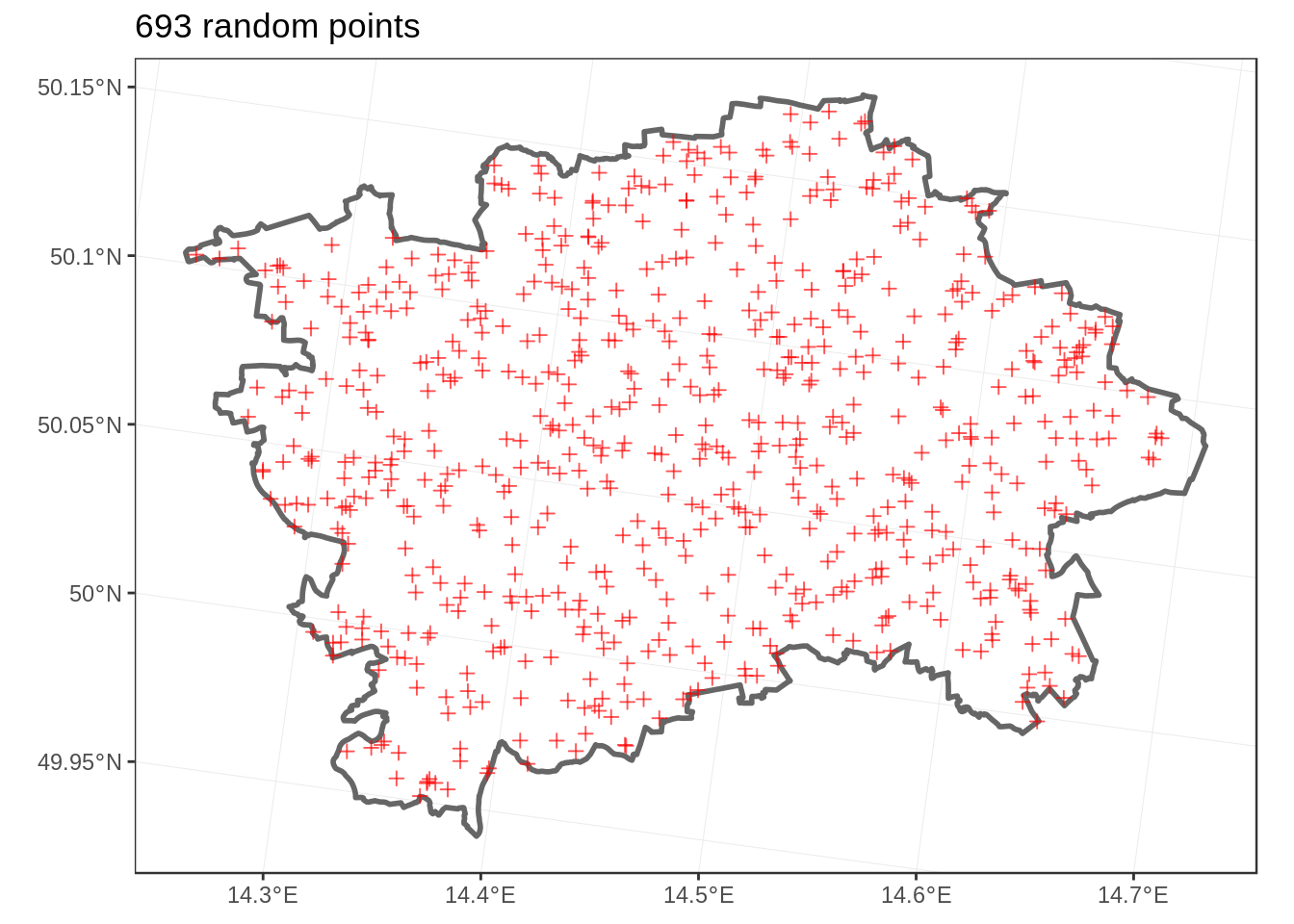
Many of the random points are close together; pruning them will be the task for the second chunk of code:
i <- 1 # iterator start

buffer_size <- 750 # minimal distance to be enforced (in meters)

repeat( {
  #  create buffer around i-th point
  buffer <- st_buffer(prazske_body[i,], buffer_size )

  offending <- prazske_body %>%  # start with the intersection of master points...
    st_intersects(buffer, sparse = F) # ... and the buffer, as a vector

  # i-th point is not really offending - it is the origin (not to be excluded)
  offending[i] <- FALSE

  # if there are any offending points left - re-assign the master points,
  # with the offending ones excluded / this is the main pruning part :)
  prazske_body <- prazske_body[!offending,]

  if ( i >= nrow(prazske_body)) {
      # the end was reached; no more points to process
      break
    } else {
      # rinse & repeat
      i <- i + 1
    }

} )

obrazek <- ggplot() +
  geom_sf(data = praha, col = 'gray40', fill = NA, lwd = 1) +
  geom_sf(data = prazske_body, pch = 3, col = 'red', alpha = 0.67) +
  theme_bw() +
  ggtitle(paste(nrow(prazske_body), 'pruned points'))

plot(obrazek)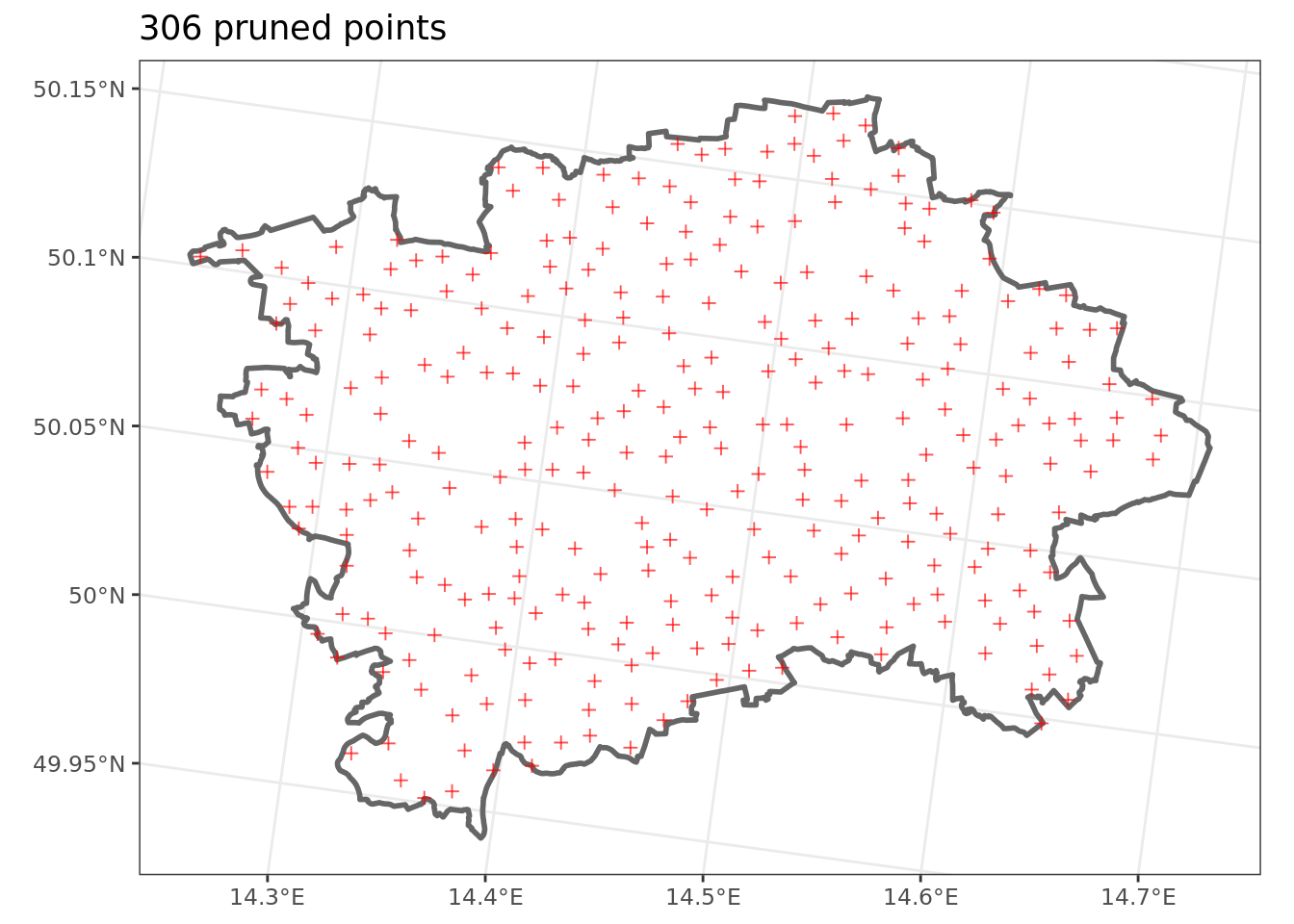
The second piece of code imposed a minimal distance around points by performing st_buffer() of size 750 meters around each point, and elimiating any offending points.
An interesting side note is that as the number of rows in the data.frame changes during calculation it is not practical to iterate via a for() cycle, but rather via repeat() and break cycle.
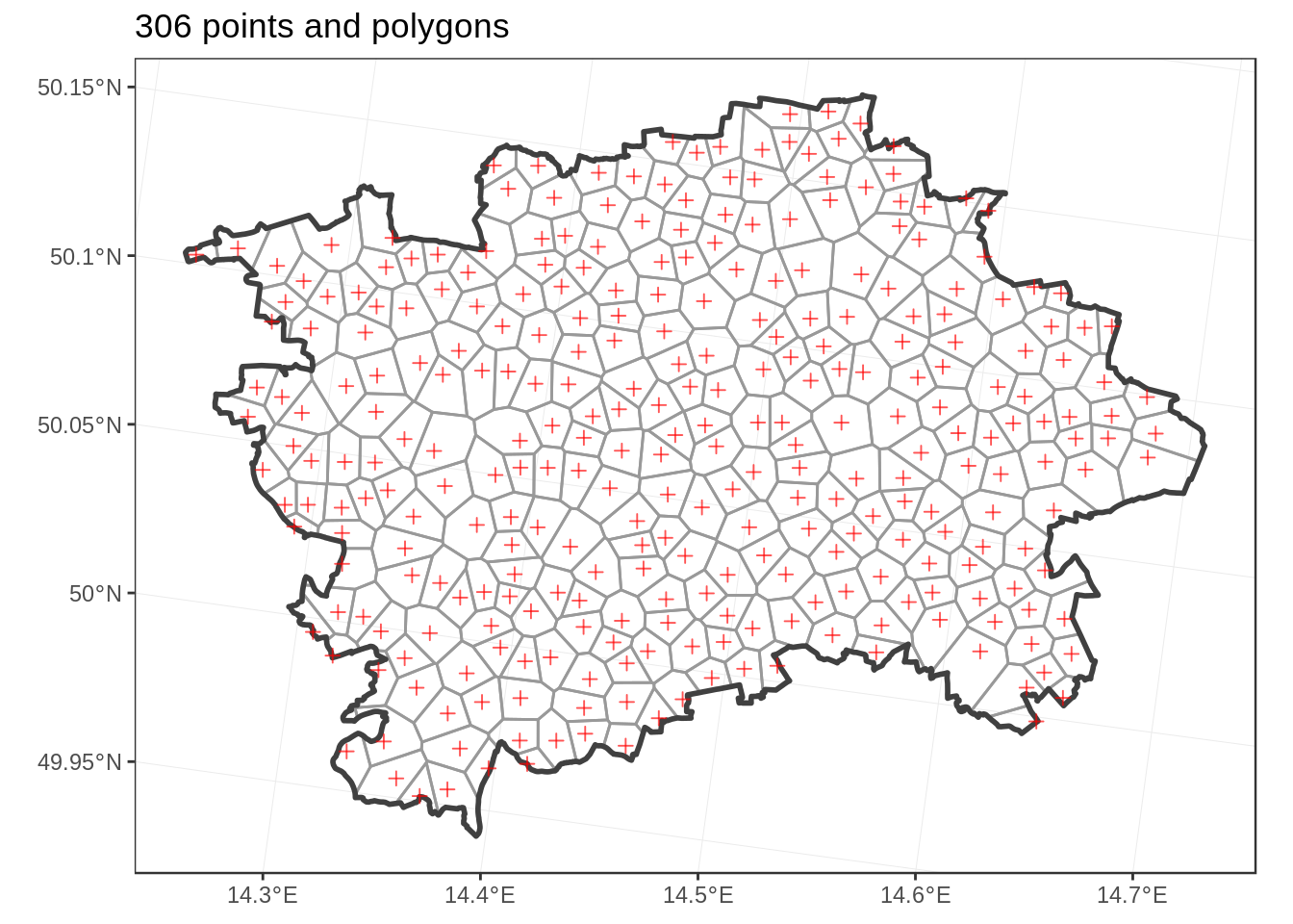
The final chunk of code performs the Voronoi tessellation & presents te result.
prazske_polygony <- prazske_body %>%  # consider the master points
  st_geometry() %>% # ... as geometry only (= throw away the data items)
  st_union() %>% # unite them ...
  st_voronoi() %>% # ... and perform the voronoi tessellation
  st_collection_extract(type = "POLYGON") %>% # select the polygons
  st_sf(crs = 5514) %>% # set metric crs
  st_intersection(praha) %>% # limit to Prague city boundaries
  st_join(prazske_body) %>% # & re-connect the data items
  st_set_agr("aggregate") # clean up

obrazek <- ggplot() +
  geom_sf(data = prazske_polygony, col = 'gray60', fill = NA) +
  geom_sf(data = praha, col = 'gray25', fill = NA, lwd = 1) +
  geom_sf(data = prazske_body, pch = 3, col = 'red', alpha = 0.67) +
  theme_bw() +
  ggtitle(paste(nrow(prazske_body), 'points and polygons'))

plot(obrazek)