I have been inspired by the work of Eliška Vlčková and Milos Popovic, who created – each in his own way – fascinating visualizations of forest cover in Europe.
Repeating of their work would be like taking owls to Athens, or coal to Newcastle, but I find the technique of extracting Land Use data from Copernicus programme greatly inspiring in other lines of work.
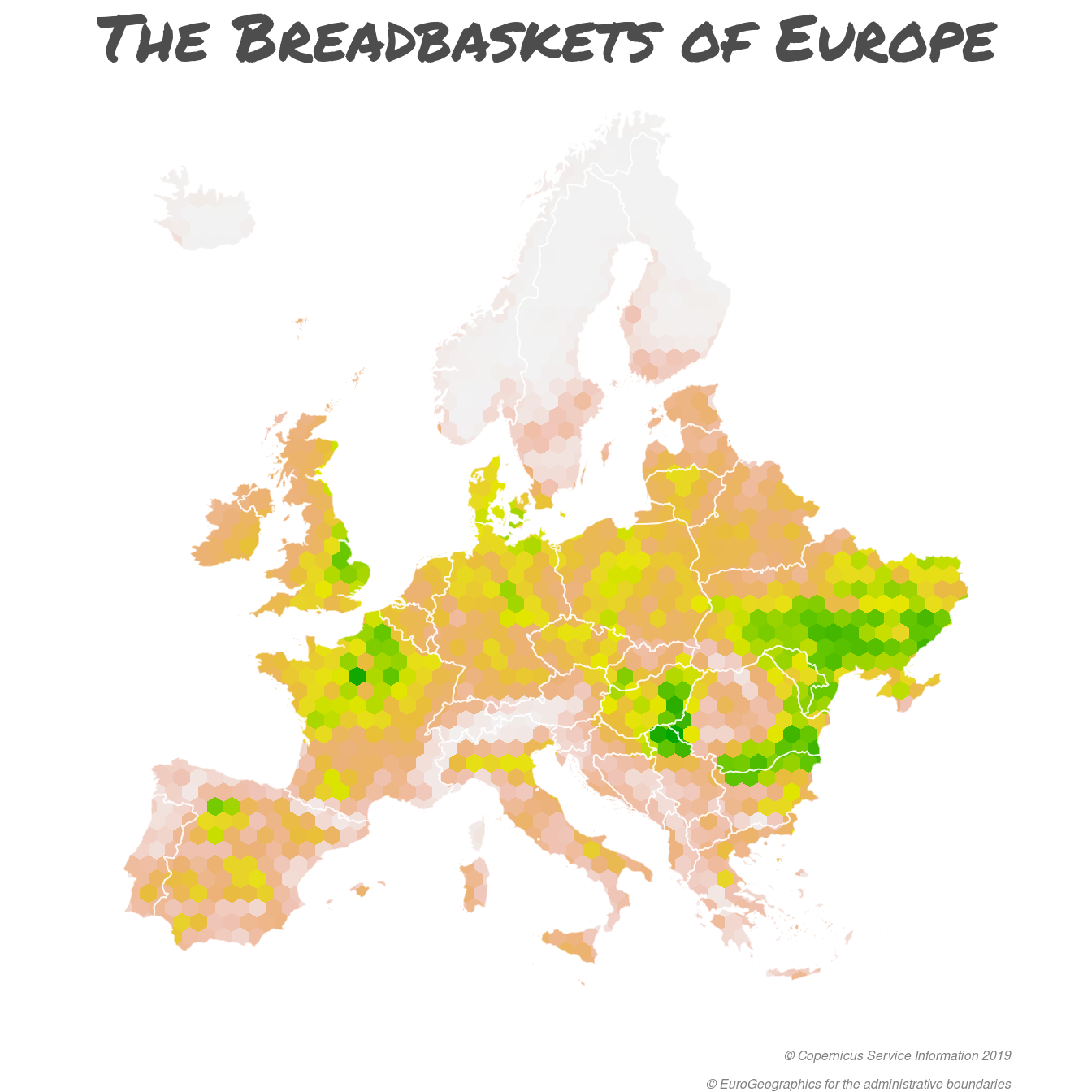
One such is identifying the breadbaskets of Europe – the areas of highest concentration of agriculture. Which can be defined as areas with the highest proportion of cropland over total area.
Cropland is a recognized land use category in Copernicus Global Land Cover product, and as it is open published it can be accessed rather easily (the only issue is file size; remote sensing rasters are big chunks of data).
library(terra)
library(ggplot2)
library(dplyr)
library(units)
library(sf)

# files of interest / remote rasters - big grid cells
remotes <- c("/E000N80/E000N80",
             "/W040N80/W040N80",
             "/W020N80/W020N80",
             "/E020N80/E020N80",
             "/E040N80/E040N80",
             "/E040N60/E040N60",
             "/W020N60/W020N60",
             "/E000N60/E000N60",
             "/E020N60/E020N60",
             "/W020N40/W020N40",
             "/E000N40/E000N40",
             "/E020N40/E020N40",
             "/E040N40/E040N40")

# files of interest / remote rasters - common parts
remotes <- paste0(
  "https://s3-eu-west-1.amazonaws.com/vito.landcover.global/v3.0.1/2019",
  remotes,
  "_PROBAV_LC100_global_v3.0.1_2019-nrt_Crops-CoverFraction-layer_EPSG-4326.tif"
  )

# if missing, download!
for (remote in remotes) {
  if(!file.exists(basename(remote))) curl::curl_download(
    url = remote,
    destfile = basename(remote)
    )
}

# one raster file to rule them all!
if(!file.exists("cropland.tif")) {
  gdalUtils::mosaic_rasters(gdalfile = basename(remotes),
                            dst_dataset = "cropland.tif",
                            of = "GTiff")
}

# read the one raster in
cropland <- rast("cropland.tif")

# a quick glance at the raw data
plot(cropland)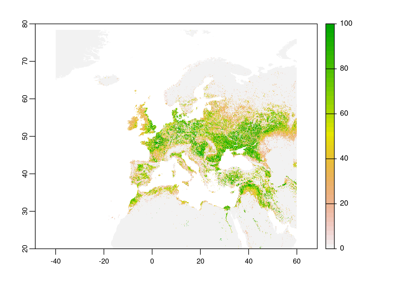
Once we have the raster side of the map it is necessary to prepare the vector part. This will consist of two parts:
- country polygons, in my case from Eurostat via
{giscoR} - hexagons, in my case generated via
sf::st_make_grid()call
An interesting problem is finding a good country polygon shapefile of continental Europe; the standard administrative approach considers French Guiana a perfectly normal part of France, and the Azores and Canary Islands of Portugal and Spain. Which is not exactly practical in my use case.
On the other hand while I am OK with not recognizing Russia as an European country a map of Europe looks wrong without the little exclave of Kaliningrad / Königsberg by the Baltics.
I thus had to resort to a little fudge, eliminating parts of France, Portugal, Spain and Russia that are too far from Bern. I was stuck with the two Spanish exclaves in Africa, but these are small enough not to be an issue at continental scale.
As I will be making areal calculation it is appropriate to project the polygons to an equal area projection; EPSG:3350 seemed a reasonable choice.
# download shapefiles from GISCO API
europe <- giscoR::gisco_get_countries(resolution = "10",
                                      region = "Europe")


# Overseas France, Azores + Canaries, and don't get me started on East Prussia!
troublemakers <- subset(europe, CNTR_ID %in% c("FR", "PT", "ES", "RU"))

buffer <- tidygeocoder::geo("Bern", quiet = T) %>%
  st_as_sf(coords = c("long", "lat"), crs = 4326) %>%
  st_buffer(as_units(1750, "km")) %>%
  st_geometry() # don't need the address column anymore

# remove the bits too far from Bern (roughly midway between Cadiz and Königsberg)
troublemakers <- troublemakers %>%
  st_intersection(buffer)

# administrative regions in equal area projection
europe <- europe %>%
  filter(!CNTR_ID %in% c("RU", "SJ", "FR", "PT", "ES")) %>%
  rbind(troublemakers) %>%
  st_transform(3035) # equal area Lambert / "European Albers"

# landmass without borders
continent <- europe %>%
  summarise() %>%
  nngeo::st_remove_holes() # get rid of funny artefacts at borders

# grid object
plocha <- as_units(5000, "km2") # target cell area

grid_spacing <- sqrt(2*plocha/sqrt(3)) %>%
  set_units("m") %>%
  as.numeric() # sf expects dimensionless spacing in crs units (= meters)

grid <- continent %>%
  st_make_grid(square = F, cellsize = c(grid_spacing)) %>% # make the grid
  st_intersection(continent) %>%
  st_sf()

plot(grid)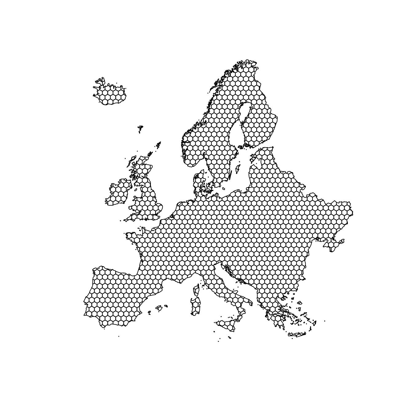
The final part of my exercise is translating the raster values to the grid object. This can be done very efficiently with the help of {exactextractr}. Since we are talking about relative measurement (proportion of cropland) mean is the most appropriate transformation.
Once the grid is populated with data the only thing remains to actually plot the data.
# extract raster values per grid cells
grid$cropland <- exactextractr::exact_extract(
  x = cropland, # input raster
  y = st_transform(grid, 4326), # target polygons, in CRS of the original raster
  fun = "mean", # transformation function; sum would give a very different result!
  progress = F # not an issue in interactive mode, but makes a mess of markdown
)

# draw the map itself
ggplot() +
  geom_sf(data = grid, aes(fill = cropland), color = NA) +
  geom_sf(data = europe, color = alpha("white", 2/3), fill = NA, lwd = 1/3) +
  scale_fill_gradientn(colors = rev(terrain.colors(7))) +
  labs(title = "The Breadbaskets of Europe",
       caption = "© Copernicus Service Information 2019
                \n© EuroGeographics for the administrative boundaries") +
  theme_void() +
  theme(legend.position = "none",
        plot.title = element_text(family = "Permanent Marker",
                                  hjust = 1/2,
                                  size = 30,
                                  color = "grey30"),
        plot.caption = element_text(face = "italic",
                                    size = 6,
                                    color = "grey50"))