On a recent Spatial Data Science across Languages workshop we discussed the problem of sharing datasets over common data analytics languages.
This topic is of a special interest to me, as I maintain a niche package of sorts, serving spatial data relevant to the Czech Republic to R users. Since the main added value of my package is curating and documenting of highly standardized open datasets the use case lends easily to a multilanguage setting – providing a language agnostic serialization pattern is implemented.
As a proof of concept I am testing serialization of German NUTS 3 regions obtained via the {giscoR} package, which interfaces the official Eurostat spatial data repository.
library(sf)

# German NUTS 3 polygons
nuesse <- giscoR::gisco_get_nuts(year = "2024",
                                 resolution = "01",
                                 country = "DE",
                                 nuts_level = 3)
# a high level overview
str(nuesse)
## Classes 'sf' and 'data.frame': 400 obs. of 10 variables:
## $ NUTS_ID : chr "DE11B" "DE11C" "DE11D" "DE121" ...
## $ LEVL_CODE : num 3 3 3 3 3 3 3 3 3 3 ...
## $ URBN_TYPE : chr NA NA NA NA ...
## $ CNTR_CODE : chr "DE" "DE" "DE" "DE" ...
## $ NAME_LATN : chr "Main-Tauber-Kreis" "Heidenheim" "Ostalbkreis" "Baden-Baden, Stadtkreis" ...
## $ NUTS_NAME : chr "Main-Tauber-Kreis" "Heidenheim" "Ostalbkreis" "Baden-Baden, Stadtkreis" ...
## $ MOUNT_TYPE: chr NA NA NA NA ...
## $ COAST_TYPE: chr NA NA NA NA ...
## $ geo : chr "DE11B" "DE11C" "DE11D" "DE121" ...
## $ geometry :sfc_MULTIPOLYGON of length 400; first list element: List of 1
## ..$ :List of 2
## .. ..$ : num [1:415, 1:2] 9.65 9.62 9.58 9.58 9.57 ...
## .. ..$ : num [1:7, 1:2] 9.53 9.53 9.54 9.54 9.54 ...
## ..- attr(*, "class")= chr [1:3] "XY" "MULTIPOLYGON" "sfg"
## - attr(*, "sf_column")= chr "geometry"
## - attr(*, "agr")= Factor w/ 3 levels "constant","aggregate",..: NA NA NA NA NA NA NA NA NA
## ..- attr(*, "names")= chr [1:9] "NUTS_ID" "LEVL_CODE" "URBN_TYPE" "CNTR_CODE" ...Germany has 400 NUTS 3 regions, and the logical way to serialize my object for use in R only would be a RDS file; this would be usable only in R environment, but is quite efficient. This will serve as my baseline.
saveRDS(nuesse, "nuts.rds")
fs::file_info("nuts.rds")$size
## 1.19MAlternative approach would be to save the dataset as an OGC GeoPackage, a platform-independent data format. A geopackage is easily accessed from any standard data analytics and GIS platform. However the format is not quite as efficient as RDS, leading to about 60% greater file size than my baseline.
write_sf(nuesse, "nuts.gpkg")
fs::file_info("nuts.gpkg")$size
## 1.91MAn interesting alternative is storing my dataset in Apache Arrow Feather file format. Out of the box it does not support spatial data features, and thus requires converting geometry to WKT.
On serialization it loses the CRS information, leaving no record what is the dimension of coordinates stored as WKT (degrees or meters, feet even?). On the other hand the compression applied is very efficient, giving us file size about one half of the RDS benchmark.
# convert geometry column to WKT string
nuesse$geom <- st_as_text(st_geometry(nuesse))

# drop the original geometry, leaving the WKT only
nuesse$geometry <- NULL

# serialize via Apache Arrow
arrow::write_feather(nuesse, "nuts.feather", compression = "zstd")
fs::file_info("nuts.feather")$size
## 600KGetting data back to R means going through the process in reverse – reading my feather file via {arrow}; it will be a regular data frame, not a spatial one. Geometry column must be reconstructed from WKT, and information on interpreting the coordinates provided externally.
# NUTS back in, under slightly different name
noix <- arrow::read_feather("nuts.feather")

# check structure - a regular data frame
str(noix)
## tibble [400 × 10] (S3: tbl_df/tbl/data.frame)
## $ NUTS_ID : chr [1:400] "DE11B" "DE11C" "DE11D" "DE121" ...
## $ LEVL_CODE : num [1:400] 3 3 3 3 3 3 3 3 3 3 ...
## $ URBN_TYPE : chr [1:400] NA NA NA NA ...
## $ CNTR_CODE : chr [1:400] "DE" "DE" "DE" "DE" ...
## $ NAME_LATN : chr [1:400] "Main-Tauber-Kreis" "Heidenheim" "Ostalbkreis" "Baden-Baden, Stadtkreis" ...
## $ NUTS_NAME : chr [1:400] "Main-Tauber-Kreis" "Heidenheim" "Ostalbkreis" "Baden-Baden, Stadtkreis" ...
## $ MOUNT_TYPE: chr [1:400] NA NA NA NA ...
## $ COAST_TYPE: chr [1:400] NA NA NA NA ...
## $ geo : chr [1:400] "DE11B" "DE11C" "DE11D" "DE121" ...
## $ geom : chr [1:400] "MULTIPOLYGON (((9.648736 49.79148, 9.61994 49.78339, 9.58053 49.77841, 9.57557 49.78151, 9.572757 49.78327, 9.5"| __truncated__ "MULTIPOLYGON (((10.16116 48.76557, 10.16414 48.77024, 10.15598 48.77164, 10.15103 48.77249, 10.15137 48.77704, "| __truncated__ "MULTIPOLYGON (((10.24128 49.05692, 10.23887 49.0536, 10.234 49.0469, 10.22182 49.04798, 10.22131 49.04803, 10.2"| __truncated__ "MULTIPOLYGON (((8.177443 48.84196, 8.16952 48.84214, 8.163085 48.84621, 8.158402 48.84665, 8.161558 48.83443, 8"| __truncated__ ...# convert back to safety of sf format, taking care of CRS
noix <- st_as_sf(noix, wkt = "geom", crs = 4326)
# a visual check
plot(noix)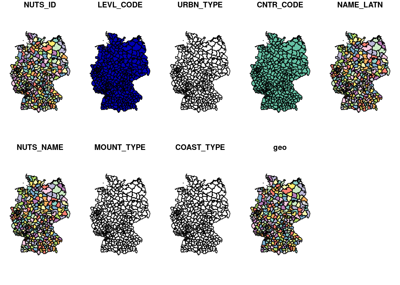
To complete the serialization POC I am reading the feather file again, this time from a python session.
First as a Shapely object via WKT, then enriching it for the CRS information that was lost on serializing and finally converting to a geopandas dataframe.
import geopandas
import pandas as pd
from shapely import wkt

# read in the dataset as a pandas dataframe
df = pd.read_feather("nuts.feather")

# restore geometry from text to WKT
df["geom"] = geopandas.GeoSeries.from_wkt(df["geom"])

# upgrade to geodataframe, re-implementing the CRS
gdf = geopandas.GeoDataFrame(df, geometry = "geom").set_crs(4326)

# a visual check
gdf.plot()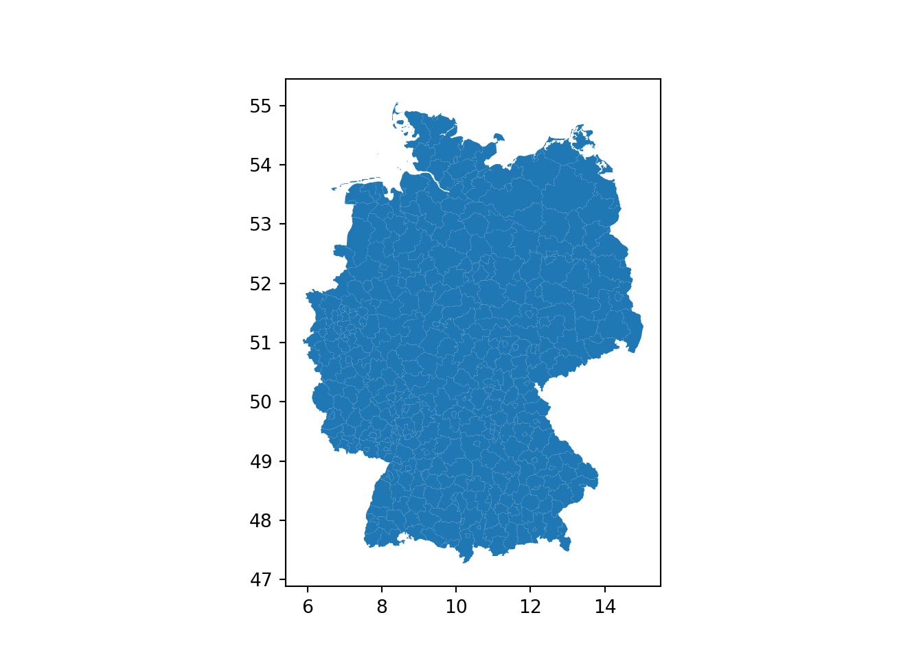
I believe I have shown the feasibility of serializing a spatial object to a relatively small Feather file, one that can be effectively consumed from both R and python setting.
The concept seems to be working, with better than expected efficiency (I would be happy to settle for a file size at par with RDS; getting to one half is a nice bonus) but some challenges remain. The chief is that the conversion from WKT is expensive, and likely would benefit from a client side caching.