While preparing an article for publication I have encountered a thorny problem: for visual consistency I needed to align legend keys between two {ggplot2} plots. Which is in theory a straightforward task, but in practice it turned out to be a bit more complicated.
The issue was that one of the plots was a choropleth map, with information keyed to the fill aesthetic, and the other was a point map. The first map turned out with classic colored squares for legend keys, while the second one with little round points. Since both legends were meant to be displayed side by side, and carry the same information, the inconsistency was a problem.
To illustrate my problem, and its eventual solution, I am using a toy example built on top of the well known & much loved nc.shp shapefile that ships with {sf} package.
library(sf)
library(ggplot2)

# the one and only NC shapefile
nc <- st_read(system.file("shape/nc.shp", package="sf"),
              quiet = T)

# three semi random counties
three_counties <- subset(nc, NAME %in% c("Ashe", "Mecklenburg", "Iredell"))
This is my first plot; note the big square legend keys.
ggplot() +
  geom_sf(data = nc) +
  geom_sf(data = three_counties,
          aes(fill = NAME)) +
  scale_fill_brewer("Counties", palette = "Set1") +
  theme_minimal()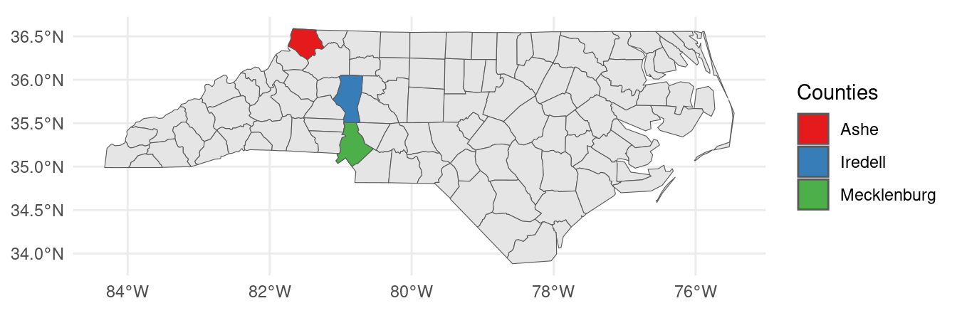
This was my second map; note the dotted legend.
ggplot() +
  geom_sf(data = nc) +
  geom_sf(data = st_centroid(three_counties),
          aes(color = NAME)) +
  scale_color_brewer("Counties", palette = "Set1") +
  theme_minimal()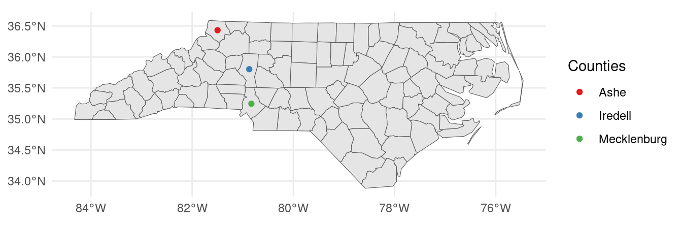
While both maps look fine the difference between style of legend keys was distracting from the fact that both legends were meant to carry the same information.
I struggled for a while, until discovering a helpful blog post by Emil Hvitfeldt on changing glyph in legend in ggplot2. The solution was to use the key_glyph argument in my geom_sf() call.
ggplot() +
  geom_sf(data = nc) +
  geom_sf(data = st_centroid(three_counties),
          aes(color = NAME),
          key_glyph = "rect") +
  scale_color_brewer("Counties", palette = "Set1") +
  theme_minimal()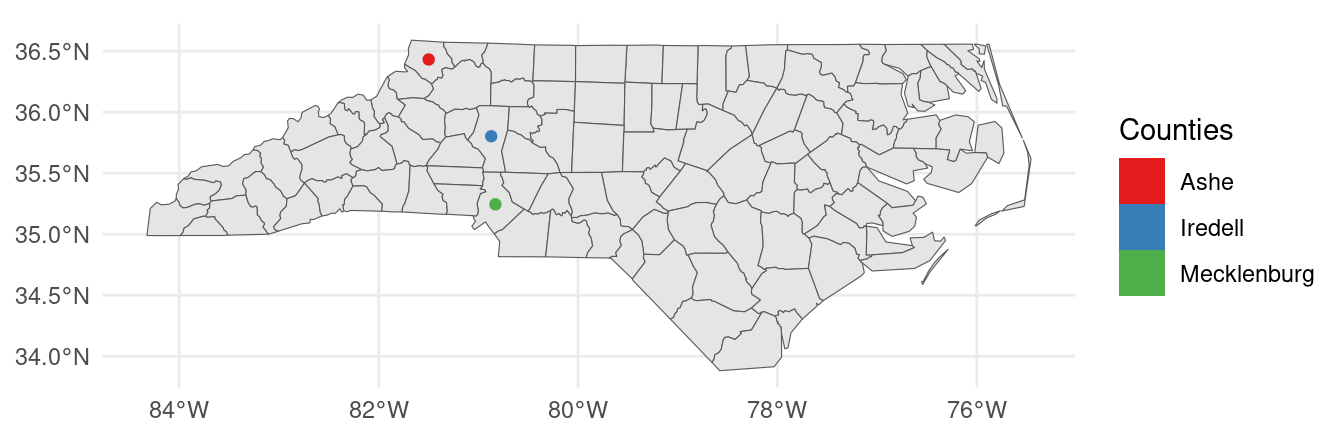
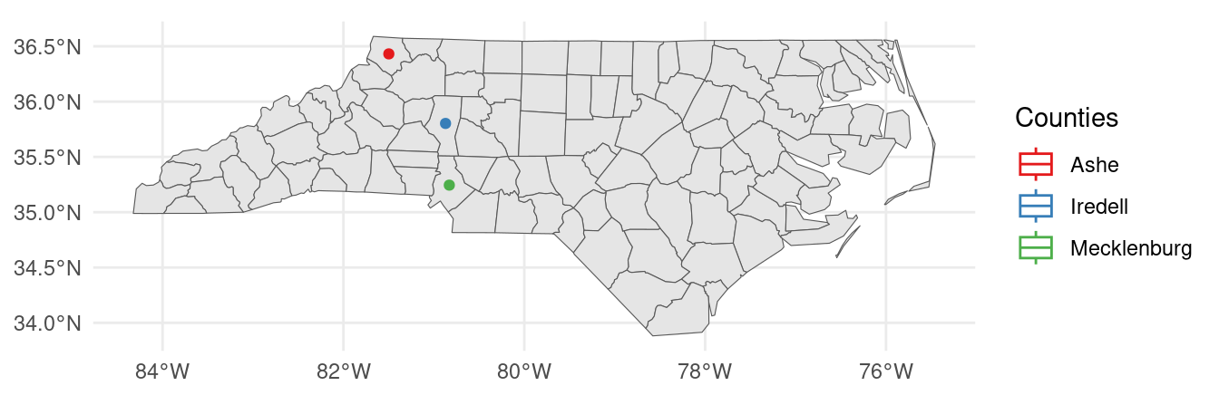
And while a plain "rect" for a rectangular key glyph turned out perfectly fine for the purpose of my article, I could not resist trying out some other options. Such as the timeseries glyph, or a little boxplot.
Which looks somewhat funky in a map settings, but will no doubt find a good use elsewhere.
ggplot() +
  geom_sf(data = nc) +
  geom_sf(data = st_centroid(three_counties),
          aes(color = NAME),
          key_glyph = "boxplot") +
  scale_color_brewer("Counties", palette = "Set1") +
  theme_minimal()