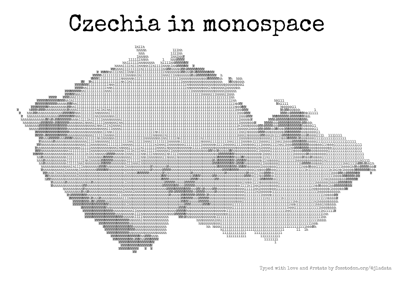
Inspired by the great Nicola Rennie of Fosstodon and her typewritten map of Scotland I have felt the need to pay her the highest form of flattery by imitating her work.
My own country felt a better start than distant Scotland, and it seemed to me as a good idea to share the code.
The first step is acquiring the raw elevation raster; I am building on the one provided by vyskopis() function of {RCzechia} package. But any DEM file read in via {terra} would do…
library(terra)   # for raster manipulation
library(ggplot2) # for plotting the plot
library(dplyr)   # for generic data frame manipulation

# raw raster - elevation of Czechia (from original DEM)
src_raster <- RCzechia::vyskopis("actual")

# a visual overview
plot(src_raster)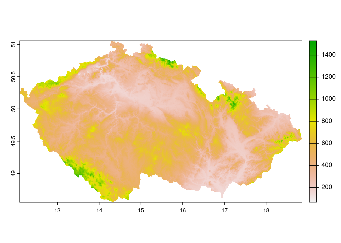
The second step is downsampling the raster drastically, so that a single raster cell will be rendered as a letter, and casting it from raster to a data frame, minding the xy argument to as.data.frame method of SpatRaster. By setting it to TRUE we will keep the coordinates of the raster cells, which will be of great help in placing our letters via ggplot2::geom_text().
I discretized the elevation to three letters - l for lowlands, h for hills and capital M for Big Mountains - via base::cut().
What turned out to be a slight challenge was plot aspect ratio; my DEM file was in geographic coordinates, and since Czechia is not quite on equator the degrees of latitude and longitude do not translate to the same distance. I was able to overcome this by getting the aspect ratio from my raster reprojected to a metric CRS (Web Mercator specifically).
The remaining fun part was finding a sufficiently old fashioned monospaced font that could plausibly pass for typewritter. I settled on Special Elite from Google Fonts.
# cast elevation from raster to data frame
map_src <- src_raster %>%
  terra::aggregate(fact = 30) %>% # downsample the raster by factor of 30
  as.data.frame(xy = T) %>% # convert raster to data frame, preserving coordinates
  mutate(category = cut(Band_1,
                        breaks = c(0, 400, 600, Inf),
                        labels = c("l", "h", "M")))

# get raster extent in meters for aspect ratio
bbox <- sf::st_bbox(project(src_raster, "EPSG:3857"))
aspect_ratio <- (bbox$ymax - bbox$ymin) / (bbox$xmax - bbox$xmin)

# now draw the rest of the map! :)
ggplot(data = map_src,
       aes(x = x, y = y, label = category)) +
  geom_text(family="Special Elite",
            size = 1.5) +
  labs(title = "Czechia in monospace",
       caption = "Typed with love and #rstats by fosstodon.org/@jladata ") +
  theme_void() +
  theme(aspect.ratio = aspect_ratio,
        plot.title = element_text(family = "Special Elite",
                                  hjust = 1/2,
                                  size = 30,
                                  color = "black"),
        plot.caption = element_text(family = "Special Elite",
                                    size = 6,
                                    color = "grey50"))