Two important concepts in the field of spatial econometrics are contiguity matrices C and weight matrices W.
Contiguity matrices provide qualitative information about which polygons are neighbors, and weight (or spatial weight) matrices give a quantitative measure of the this neighborhood relationship.
In this post I provide several alternative approaches to constructing contiguity and weight matrices, with examples using the well known and much loved nc.shp shapefile that ships with the {sf} package.
Both contiguity and weight matrices are implemented in the {spdep} package, which is the de-facto standard approach to spatial dependence modelling in R settings.
The contiguity matrix is implemented as
nb(short for neighborhood) object, which is a list of indexes of objects considered neighbors (whatever that means in a given context).The weights matrix is implemented as
listwobject, which is a compound consisting of two items:neighboursobject, which is in principle the same as anbobject, and aweightsobject, which contains the weights matrix itself.
Formally the weight matrix encodes the neighborhood structure as a n × n matrix W, where elements wi,j are the spatial weights:
\[ {\bf W} = \left(\begin{array}{ccccc} w_{1,1}&w_{1,2}&w_{1,3}&\cdots &w_{1,n}\\ w_{2,1}&w_{2,2}&w_{2,3}&\cdots &w_{2,n}\\ w_{3,1}&w_{3,2}&w_{3,3}&\cdots &w_{3,n}\\ \vdots&&&\ddots&\\ w_{n,1}&w_{n,2}&w_{n,3}&\cdots &w_{n,n} \end{array}\right) \] The weights wi,j have value of zero for polygons that are not considered neighbors, and non–zero values for neighboring ones.
By convention a polygon is not considered to be neighboring with itself, so the diagonal of a weights matrix is zero by definition.
Also by convention the individual weights are row standardized, so that weight matrix rows sum to 1. Consequently the matrix itself sums to the number of observations n. This convention is represented as style='W' in the framework of {spdep} models (other conventions, such as standardizing all weights to unity, are possible, but less commonly used).
My first step is loading required packages and the nc.shp shapefile as counties object. The shapefile is then projected to a feety CRS, because as an European, metric born & bred, I find the quaint local customs amusing.
library(spdep)
library(dplyr)
library(sf)
library(ggplot2)

# NC counties as polygons - a shapefile shipped with the sf package
counties <- st_read(system.file("shape/nc.shp", package = "sf"), quiet = T) %>%
  st_transform(2264) # a feety CRS, to make it more interesting :)
My second step is preparing a convenience function report_results() in order to plot a map illustrating the calculated results. It takes for argument a listw object, and draws a plot of neighbors of a single county, with neighborhood weight as labels. Notice that the labels are placed in the centroid of the neighbor.
This convenience function will be used to show differences in calculated matrices (because a graphical example is more than 1000 words, and because I dislike repeating my code).
County Franklin makes for a good example, because out of all the North Carolina counties it has the biggest difference between rook and queen neighborhoods (it touches neighboring counties Halifax and Johnston in single point each).
# a convenience function; will display county Franklin & its neighbors
report_results <- function(listw_object) {

  chart_source <-  counties %>%
    # selects neigbbors of cnty Franklin (only) as polygons
    slice(purrr::pluck(listw_object$neighbours,
                       which(counties$NAME == "Franklin"))) %>%
    # new column of weights relative to cnty Franklin
    mutate(weight = purrr::pluck(listw_object$weights,
                               which(counties$NAME == "Franklin")))

  # draw a plot based on chart_source object
  ggplot(data = chart_source) +
    geom_sf() +
    geom_sf_label(aes(label = scales::percent(weight, accuracy = 1)),
                  # let's use the label to mark county centroid!
                  fun.geometry = sf::st_centroid) +
    # centroid of cnty Franklin, for reference
    geom_sf(data = st_centroid(counties[which(counties$NAME == "Franklin"), ]),
            color= "red", pch = 4) +
    theme_void()

}
The first example is creating a queen style neighborhood, in which neighbors are defined as polygons (counties) sharing at least a single point. In this framework county Franklin has 7 neighbors, giving each equal 14% neighborhood weight (where 14.29% = 100 / 7).
The call to invoke queen neighborhoods is spdep::poly2nb() with queen argument set to TRUE (which is the default).
queen_hoods <- st_geometry(counties) %>%
  poly2nb(queen = TRUE) %>%
  nb2listw()

report_results(queen_hoods)
The second approach is creating a rook style neighborhood, in which neighbors are defined as polygons (counties) sharing an edge – a single point is not enough. In this framework county Franklin has 5 neighbors, giving each weight of 20%.
In practice, when dealing with polygons that originated from a sufficiently random process – such as admin areas that originated “bottom up” in a long settled area – you will find very few, if any, differences between queen and rook neighbors. Cases such as the famous four corners point between Utah, Arizona, Colorado and New Mexico are rather rare, occurring chiefly in “top down” driven administration of newly settled territories; a fine example being the US State of Iowa.
I confess that I had to cheat a bit using setdiff() on the two nb objects to find a sufficiently salient example in a mostly organically settled state of North Carolina, as I really wanted to stick with the nc.shp shapefile we all know and love.
The call to invoke rook neighborhoods is spdep::poly2nb() with queen argument set to FALSE (meaning a rook is the not queenly approach).
rook_hoods <- st_geometry(counties) %>%
  poly2nb(queen = FALSE) %>% # not queen means rook
  nb2listw()

report_results(rook_hoods)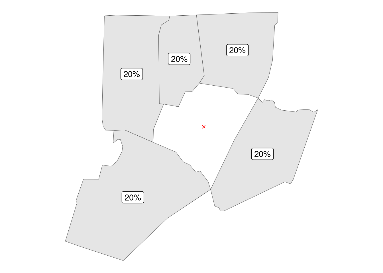
Third approach is basing neighborhoods on K nearest neighbors. This approach is not defined for polygons (for good reasons) but a good practice for point data.
In order to make it work for polygons these have to be first converted to points via sf::st_centroid(). In this framework county Franklin (and every other, by definition) has 3 neighbors, giving each weight of 33%.
The call to invoke KNN neighbors is spdep::knearneigh(), where argument k is the desired number of neighbors.
knn_hoods <- st_geometry(counties) %>%
  st_centroid() %>% # polygons to points
  knearneigh(k = 3) %>% # always 3 neighbors - never more, never less...
  knn2nb() %>%
  nb2listw()

report_results(knn_hoods)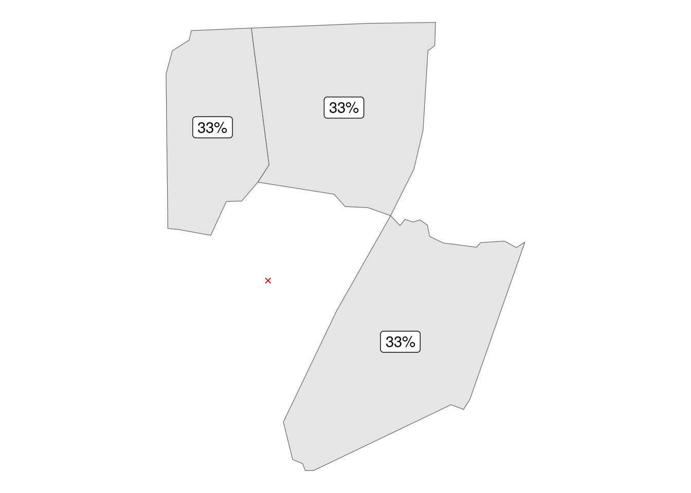
Fourth approach is basing neighborhoods on distance. This approach is again defined for points only, so in order to use it we have to convert our polygons to centroids.
In this framework we have to set the minimum (usually zero) and maximum distance; I am using 50 miles as maximum distance between county centroids to be considered “neighboring”.
In this framework county Franklin has 12 neighbors, giving each 8% weight (where 8.33% = 100 / 12).
The call to invoke distance based neighbors is spdep::dnearneigh(), where argument d1 is the minimal, and d2 the maximal distance.
distance_hoods <- st_geometry(counties) %>%
  st_centroid() %>% # polygon to points
  dnearneigh(d1 = 0, # from zero...
             d2 = 5280 * 50) %>% # ... to 50 miles
  nb2listw()

report_results(distance_hoods) 
Important fine tuning technique is altering the weights of your listw object. Depending on your use case it may be – and may not be – appropriate to give each neighbor equal weight, such as the 8% used in the last example. Or there may be a compelling reason to make some neighbors less equal than others.
Fortunately, the weights element of your listw object can be easily rewritten as your situation requires.
A common approach is to apply inverse distance weighting, giving more prominence to close neighbors and less to far off ones. Note how the weight of close neighbors moves from 8% to 13%, and drops to 5% for the farthest one.
For this frequent use case we can leverage the spdep::nbdists() function that calculates distances between elements of a nb neighborhood object.
# start with a nb object (not yet listw)
nblist <- st_geometry(counties) %>%
  st_centroid() %>%
  dnearneigh(d1 = 0,d2 = 5280 * 50)

# then use the nb object to create a listw object
idw_hoods <- nb2listw(nblist)

# then rewrite the "weights" part of the said listw object
# using information contained in the original nb
idw_hoods$weights <- nbdists(nblist,
                             st_coordinates(st_centroid(counties))) %>%
  lapply(function(x) 1/x)  %>% # distance inverted
  lapply(function(x) x/sum(x)) # W-style standardization


report_results(idw_hoods)
Yet more aggressive approach is basing weights on inverse of squared distances; notice how the weight of Nash County increases to 20%, while the weight of Orange County drops to 3%.
nblist <- st_geometry(counties) %>%
  st_centroid() %>%
  dnearneigh(d1 = 0,d2 = 5280 * 50)

idwsq_hoods <- nb2listw(nblist)

# again, rewrite the existing weights part of listw object
idwsq_hoods$weights <- nbdists(nblist,
                              st_coordinates(st_centroid(counties))) %>%
  lapply(function(x) 1/(x^2)) %>% # square of distance inverted
  lapply(function(x) x/sum(x)) # W-style standardization

report_results(idwsq_hoods)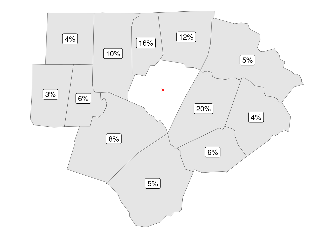
A different approach is creating weights based on the length of shared border; this requires slightly more coding, as there is no standard function to return a list of border lengths of a nb set (unlike for the list of distances), but not overly so.
Note how, by basing the border length weighted list on queen neighborhoods, we end up with zero weights for the “joinded in the corners” counties, effectively removing the difference between the queen and the rook neighborhood patterns.
# start with a queen style, rather than rook style nb object
# - it will make the zeroes in corners (zero length border) really stand out
nblist <- st_geometry(counties) %>%
  poly2nb(queen = TRUE)

# then create a listw object
borderline_hoods <- nb2listw(nblist)

# then pre-allocate a list of distances
distances <- vector("list", length(nblist))

# use i as iterator over list of distances
for (i in seq_along(distances)) {

  # indices of neighbors of i-th element
  neighbor_ids <- purrr::pluck(nblist[[i]])

  # shared borders of (multiple) neighbors and i-th element as a line
  distances[[i]] <- st_intersection(st_geometry(counties)[neighbor_ids],
                                    st_geometry(counties)[i]) %>%
    st_length() %>% # from line as geometry to length of said line
    units::drop_units() # we want share of total, which is unitless

}

# apply the W style standardization
distances <- lapply(distances, function(x) x/sum(x))

# overwrite the original weights object
borderline_hoods$weights <- distances

report_results(borderline_hoods)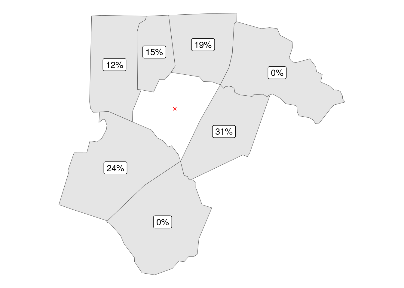
I believe I have demonstrated both:
- the variety of options for calculating the contiguity and weight matrices
- the ease of doing so within the context of
{spdep}package and friends
QED :)